naniar version 0.3.1 “Strawberry’s Adventure” is now on CRAN, hooray!

Strawberry the cab horse turning into Fledge, the Pegasus, the first talking animal of Narnia

naniar is an R package that makes it easier to explore, analyse, and visualise missing data and imputed values. It is designed to be tidyverse-friendly, so it works fluidly in an analysis workflow.

I encountered some pretty gnarly missing data when I first started my PhD, which was really frustrating. I wanted to do something about it, and the naniar package is the realisation of that frustration. naniar aims to make it easy to do the following:

1. Find if there is missing data, and how much there is.
2. Clean up, tidy, and recode missing values
3. Explore why data is missing
4. Evaluate imputed values

I’ve written in more detail about how to get started with missing data in this “getting started”. If you are not familiar with the naniar package, I would recommend starting there for a quick tour of its features.

There were a few things that changed in this release, some of them big, some small, and some technical, let’s break them down now.

Visualising patterns of missingness

Alberto Triano

Visualising the different co-occurrences of missingness is tricky. This is where you want to show where there are cases or variables that have the same number of missings. You can now visualise these missingness patterns using upset plots from UpSetR package¹. To create these, you need to get the data into the right format using as_shadow_upset, and then call UpSetR:

library(naniar)
library(ggplot2)

riskfactors %>%
    as_shadow_upset() %>%
    UpSetR::upset()

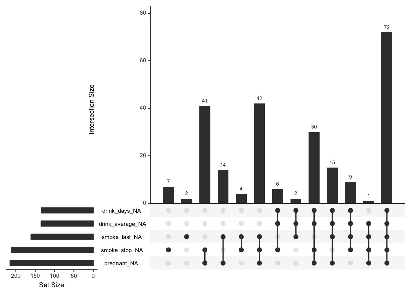
On the left is a plot of the number of missings in each individual variable (missingness is indicated here with variable_NA), and then on the right we have the size of the missingness in the combinations of variables. So here we see that out of the variables selected, the largest number of missings is about 72. This means that there are 72 rows where all five of these variables are missing. You can decide to look at more possible sets of missings by changing the nsets option in upset to be the same as the number of variables with missings - using the new n_var_miss function:

risk_n_var_miss <- n_var_miss(riskfactors)

riskfactors %>%
    as_shadow_upset() %>%
    UpSetR::upset(nsets = risk_n_var_miss)

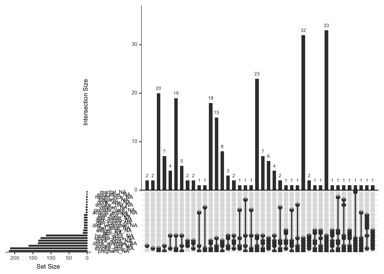
There are more missingness patterns, and this one is a little tricky to read, so use wisely!

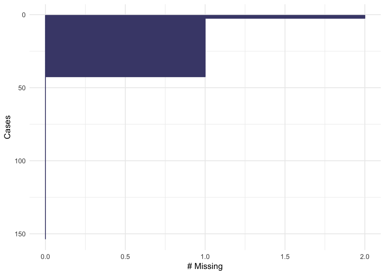
New colours for gg_miss_case and gg_miss_var

The default colour for gg_miss_case and gg_miss_var is now a lorikeet purple , taken from from ochRe package. Previously, gg_miss_case was light grey, which had poor contrast against a white background. gg_miss_var had a different colour for each variable, which I found unnecessary. Additionally, gg_miss_case is ordered by the most missing cases at the top, and also gains a show_pct option for the x axis, to be consistent with gg_miss_var #153.

gg_miss_case(airquality)

gg_miss_var(airquality)

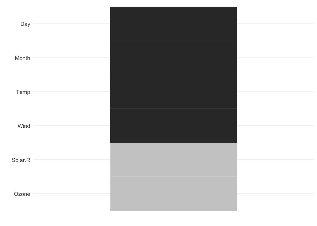
gg_miss_which shows us which variables have missings - it has been is rotated 90 degrees so it is easier to read variable names

gg_miss_which(airquality)

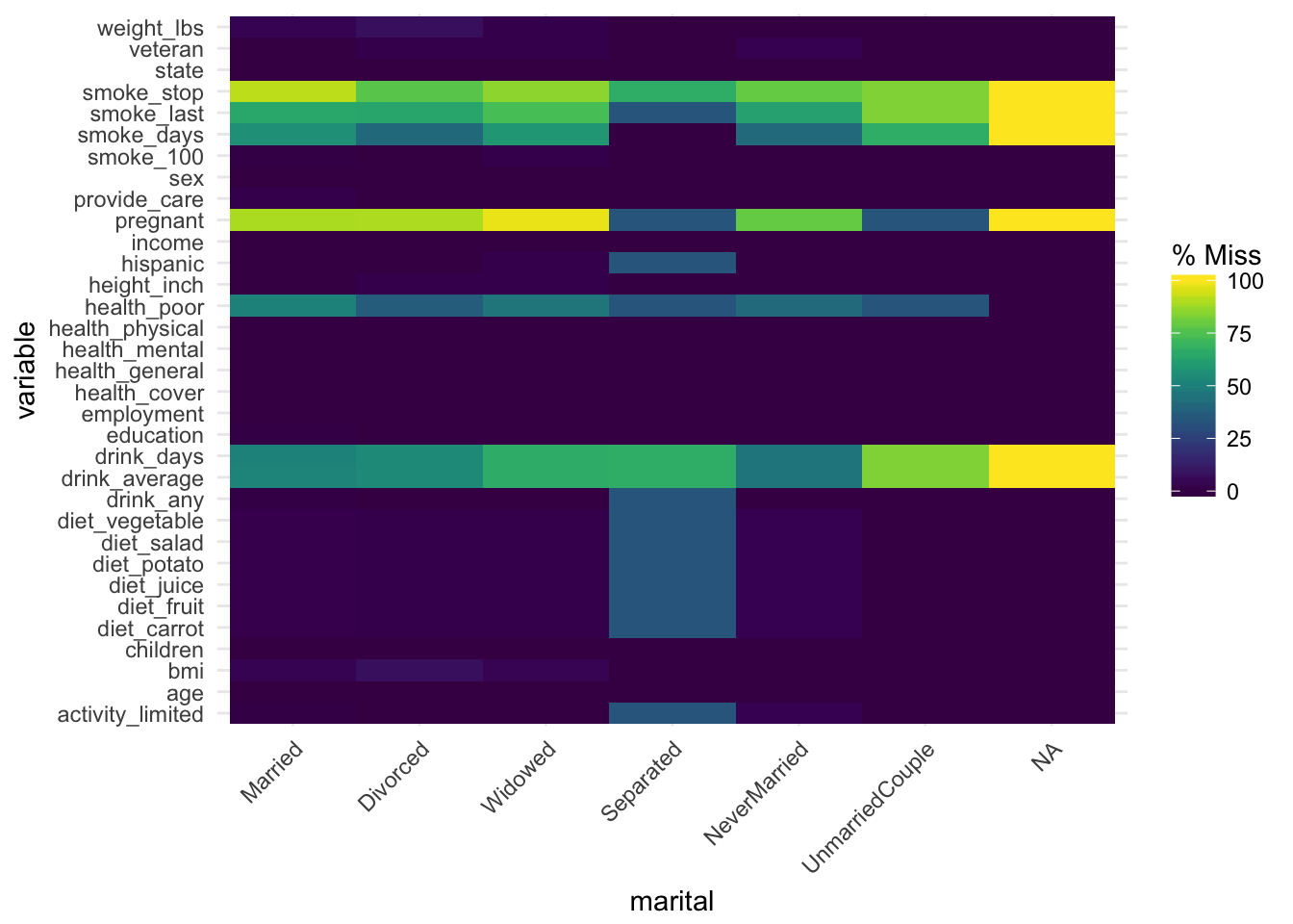
gg_miss_fct now uses a minimal theme and tilts the axis labels #118. This plot shows us the amount of missings in each column of a dataset for a given factor.

gg_miss_fct(x = riskfactors, fct = marital)

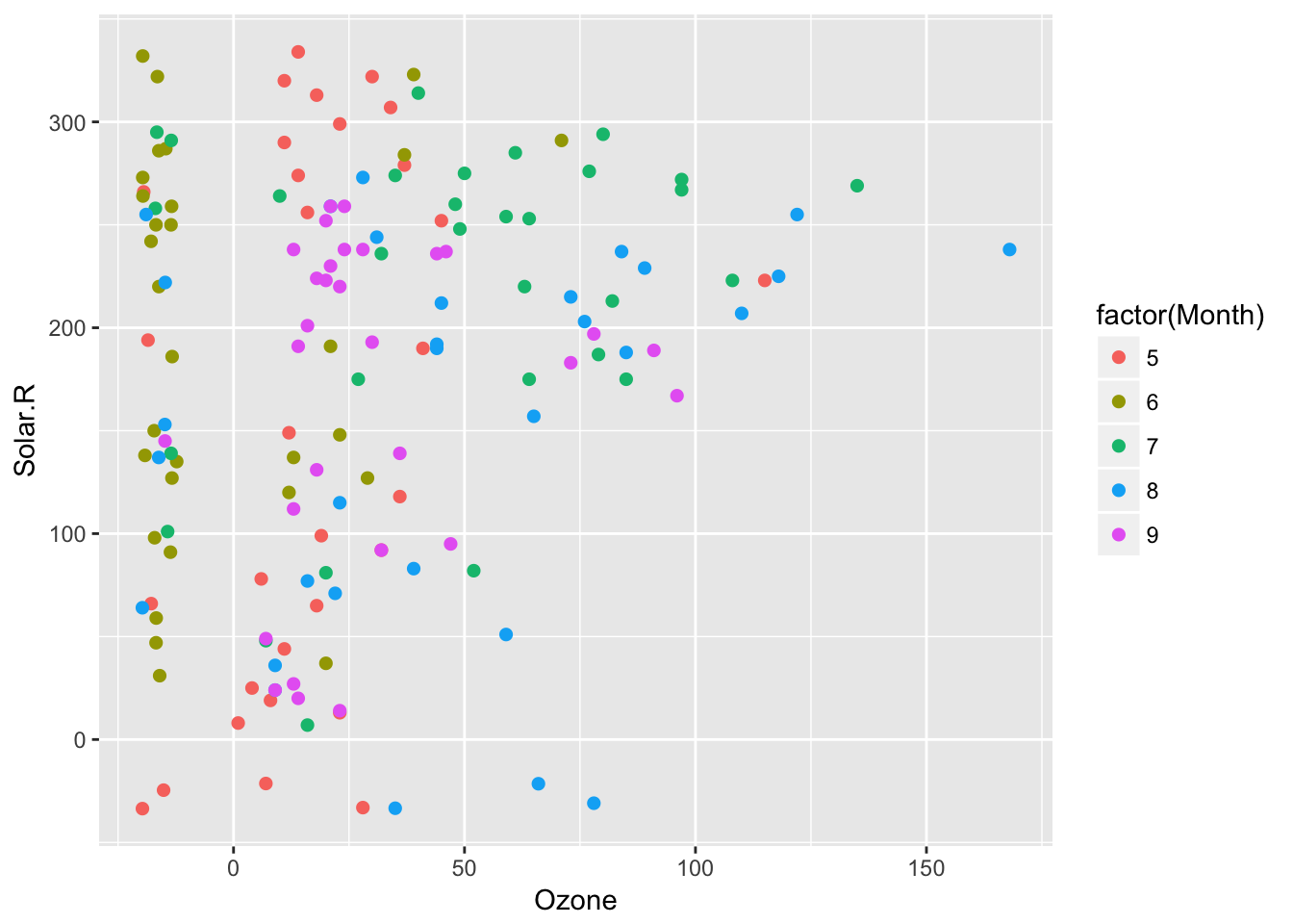
Aesthetics now map as expected in geom_miss_point(). This means you can write things like geom_miss_point(aes(colour = Month)) and it works appropriately. This was fixed by Luke Smith in #144, fixing #137. This removes the colouring provides by default, as it is overridden.

ggplot(airquality,
       aes(x = Ozone,
           y = Solar.R,
           colour = factor(Month))) +
  geom_miss_point()  

List common types of missing.

There are a ton of “gotcha’s” when it comes to missing data, and I find myself often feeling like this:

One that is rather frustrating is when there are hidden NA values lurking. Some notable examples are: " NA” and “NA “, and “N/A”. common_na_strings is a vector of possible NA strings to watch out for, and common_na_numbers is a vector of possible NA numbers to be wary of:

common_na_strings

##  [1] "NA"     "N A"    "N/A"    "NA "    " NA"    "N /A"   "N / A" 
##  [8] " N / A" "N / A " "na"     "n a"    "n/a"    "na "    " na"   
## [15] "n /a"   "n / a"  " a / a" "n / a " "?"      "."      "NULL"  
## [22] "null"   ""       "."

common_na_numbers

## [1]    -9   -99  -999 -9999  9999    66    77    88

These can be combined to look for unusual missing values in a dataset with miss_scan_count:

 dat_ms <- tibble::tribble(~x,  ~y,    ~z,
                          1,   "A",   -100,
                          3,   "N/A", -99,
                          NA,  NA,    -98,
                          -99, "E",   -101,
                          -98, "F",   -1)

 miss_scan_count(dat_ms,c(-99,-98))

## # A tibble: 3 x 2
##   Variable     n
##   <chr>    <int>
## 1 x            2
## 2 y            0
## 3 z            2

 miss_scan_count(dat_ms,c("-99","-98","N/A"))

## # A tibble: 3 x 2
##   Variable     n
##   <chr>    <int>
## 1 x            2
## 2 y            1
## 3 z            2

 miss_scan_count(dat_ms,common_na_strings)

## # A tibble: 3 x 2
##   Variable     n
##   <chr>    <int>
## 1 x            4
## 2 y            4
## 3 z            5

 miss_scan_count(dat_ms,common_na_numbers)

## # A tibble: 3 x 2
##   Variable     n
##   <chr>    <int>
## 1 x            2
## 2 y            0
## 3 z            2

Or used in replace_with_na (but use with caution!!!)

dat_ms %>%
  replace_with_na_all( ~.x %in% common_na_strings)

## # A tibble: 5 x 3
##       x y         z
##   <dbl> <chr> <dbl>
## 1     1 A      -100
## 2     3 <NA>    -99
## 3    NA <NA>    -98
## 4   -99 E      -101
## 5   -98 F        -1

dat_ms %>%
  replace_with_na_all( ~.x %in% common_na_numbers)

## # A tibble: 5 x 3
##       x y         z
##   <dbl> <chr> <dbl>
## 1     1 A      -100
## 2     3 N/A      NA
## 3    NA <NA>    -98
## 4    NA E      -101
## 5   -98 F        -1

Imputation

Samuel Zeller

Some simple imputation functions have been added into naniar. These are not what I would recommend using to draw inferences, but instead something to explore structure in the missingness, and to actually visualise missing values.

The are two main imputation functions that have been added:

• impute_below, and
• impute_mean.

impute_below imputes values below the range of the data, so that they can be visualised. This is similar to shadow_shift, but framed at a whole dataframe - so it works for every column of a dataframe. impute_mean imputes the mean, and for factors will imputes the mode, randomly choosing a tie breaker if there is a tie.

impute_below and impute_mean each have scoped variants that work for specific named columns, _at and _if, and _all for columns that satisfy some predicate function.

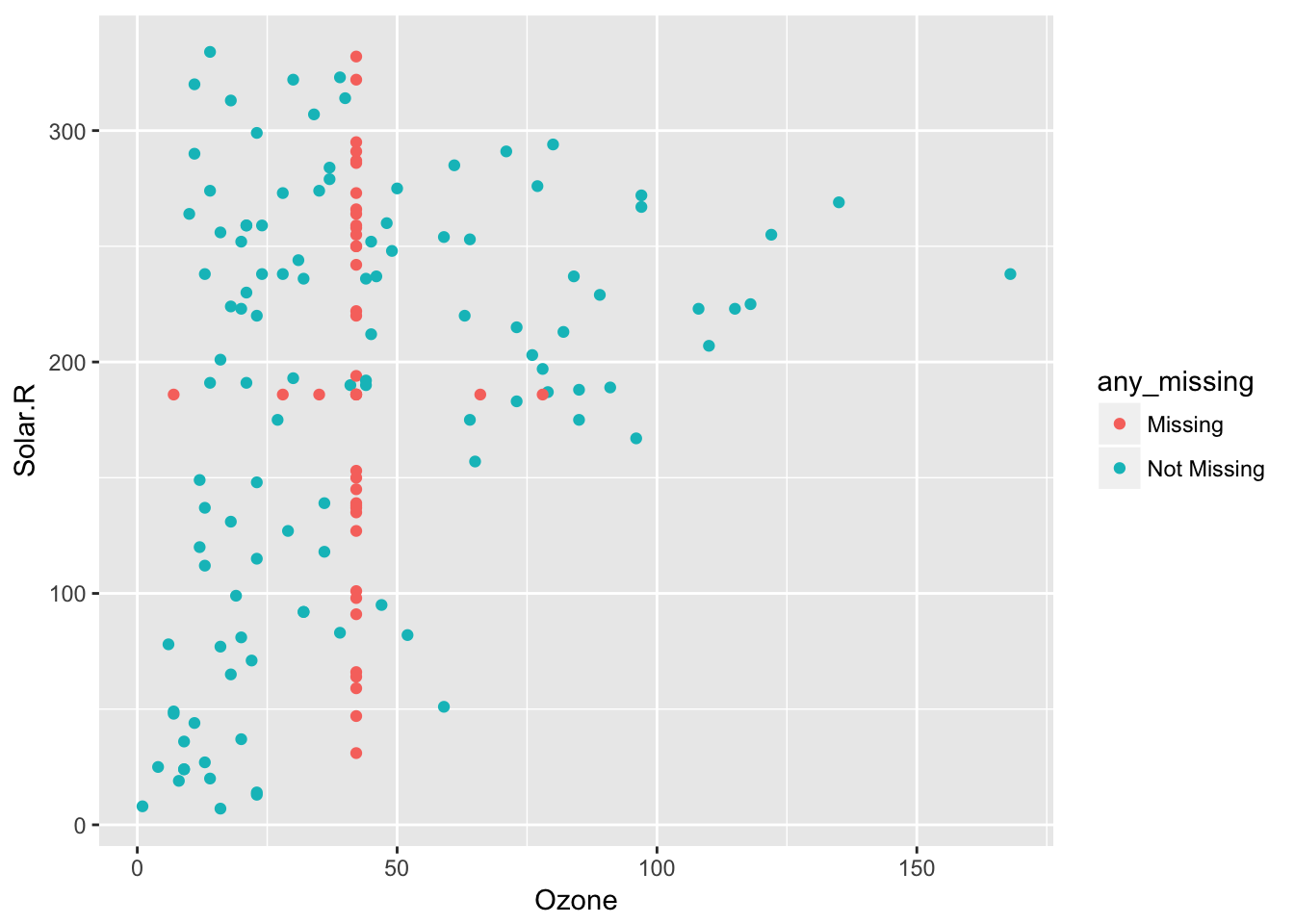
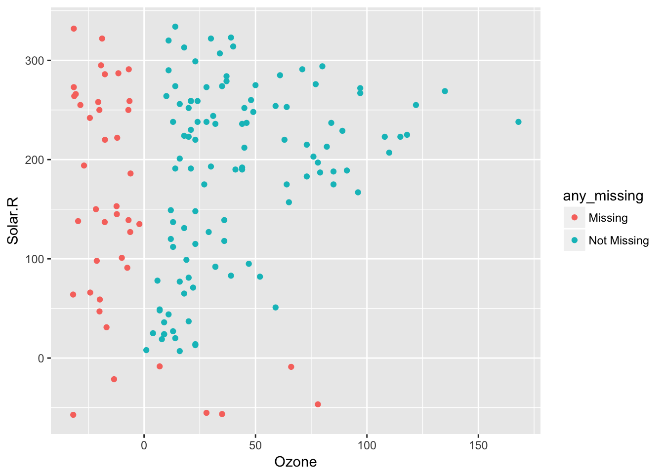
This means impute_below_at can be used for specified columns, and impute_below_if will be applied on columns that satisfy some condition. For example, is.numeric. We can impute the mean for only numeric data, using bind_shadow and add_label_shadow to track the missing values so we can plot them:

airquality %>%
  bind_shadow() %>%
  add_label_shadow() %>%
  impute_mean_if(is.numeric) %>%
  ggplot(aes(x = Ozone,
             y = Solar.R,
             colour = any_missing)) + 
    geom_point()

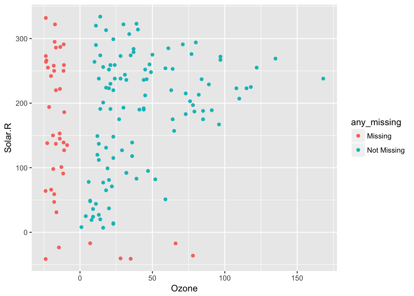
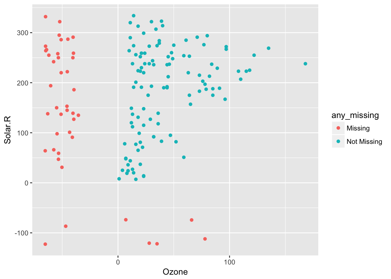
impute_below Performs as for shadow_shift, but performs on all columns (impute_below doesn’t have an _all suffix). This means that it imputes missing values 10% below the range of the data (powered by shadow_shift), to facilitate graphical exploration of the data. In addition to this, impute_below and shadow_shift gain arguments prop_below and jitter, to control the degree of shift, and also the extent of jitter.

So 10% jitter (default)

airquality %>%
  bind_shadow() %>%
  impute_below(jitter = 0.1) %>%
  add_label_shadow() %>%
  ggplot(aes(x = Ozone,
             y = Solar.R,
             colour = any_missing)) + 
    geom_point()

So 20% jitter

airquality %>%
  bind_shadow() %>%
  impute_below(jitter = 0.2) %>%
  add_label_shadow() %>%
  ggplot(aes(x = Ozone,
             y = Solar.R,
             colour = any_missing)) + 
    geom_point()

And 20% jitter plus 20% below:

airquality %>%
  bind_shadow() %>%
  impute_below(jitter = 0.20,
               prop_below = 0.30) %>%
  add_label_shadow() %>%
  ggplot(aes(x = Ozone,
             y = Solar.R,
             colour = any_missing)) + 
    geom_point()

Handy Helpers

“Handy Helpers” are functions that make some small tasks with missing data more consistent and straightforward. This includes functions that extend from of anyNA and generalise to any and all cases, and also work for complete data. This means we have the functions:

• all_miss() / all_na() equivalent to all(is.na(x))
• any_complete() equivalent to all(complete.cases(x))
• any_miss() equivalent to anyNA(x)

For example:

all_miss(airquality)

## [1] FALSE

all_miss(mtcars)

## [1] FALSE

any_miss(airquality)

## [1] TRUE

any_miss(mtcars)

## [1] FALSE

any_complete(airquality)

## [1] TRUE

any_complete(mtcars)

## [1] TRUE

We also now have complete complements to functions #150:

• miss_var_pct – complete_var_pct
• miss_var_prop – complete_var_prop
• miss_case_pct – complete_case_pct
• miss_case_prop – complete_case_prop

There are now helpers to remove data or the shadow part of a dataframe, with unbind_shadow and unbind_data. This is handy in cases where you add the shadow to the data with bind_shadow, do some analysis, and then you might want to discard the shadow or the data. For a recap on what shadows are and why they are useful in missing data analysis, see this section on the getting started vignette.

Imported is_na and are_na from rlang. These are different to base R’s is.na, in that is_na return a logical vector of length 1 (does this thing contain missings?), and are_shadow returns a logical vector of length of the number of names of a data.frame, more similar to is.na(). from base R.

is_na(airquality)

## [1] FALSE

are_na(airquality) %>% head()

##      Ozone Solar.R  Wind  Temp Month   Day
## [1,] FALSE   FALSE FALSE FALSE FALSE FALSE
## [2,] FALSE   FALSE FALSE FALSE FALSE FALSE
## [3,] FALSE   FALSE FALSE FALSE FALSE FALSE
## [4,] FALSE   FALSE FALSE FALSE FALSE FALSE
## [5,]  TRUE    TRUE FALSE FALSE FALSE FALSE
## [6,] FALSE    TRUE FALSE FALSE FALSE FALSE

There are also is_shadow and are_shadow functions, to determine if something contains a shadow column. Similar to rlang::is_na and rland::are_na, is_shadow This might be revisited at a later point to reflect values inside the shadow columns - “shadow values” as “shades”. See is_shade and any_shade in add_label_shadow.

is_shadow(airquality)

## [1] FALSE

are_shadow(airquality)

## [1] FALSE FALSE FALSE FALSE FALSE FALSE

aq_bind <- bind_shadow(airquality)
is_shadow(aq_bind)

## [1] TRUE

are_shadow(aq_bind)

##  [1] FALSE FALSE FALSE FALSE FALSE FALSE  TRUE  TRUE  TRUE  TRUE  TRUE
## [12]  TRUE

Added miss_var_which, to lists the variable names with missings

miss_var_which(airquality)

## [1] "Ozone"   "Solar.R"

Minor Changes

miss_var_summary and miss_case_summary now return use order = TRUE by default, so cases and variables with the most missings are presented in descending order. Fixing #163

Added some detail on alternative methods for replacing with NA in the vignette replacing values with NA.

Future work

Daniel Cheung

The next release of naniar 0.4.0 (codenamed “An Unexpected Meeting”) will feature alternative flavours of missing value, something that I have been thinking about for a while now, performance improvements, and adding more vignettes. You can see my current plan at the 0.4.0 milestone here, it should be out before UseR! in Brisbane, which starts on the 10th July.

Thanks

Thank you to everyone who has contributed to this package, whether it is with code, or issues or pull requests, over the course of the past (nearly 2!) years, you are all great!

• Di Cook
• Miles McBain
• Colin Fay
• Romain François
• Jim Hester
• Luke Smith
• Earo Wang
• Stuart Lee
• Jessica Minnier
• Stephanie Zimmer
• Eric Nantz

If anyone has any feedback, please feel free to file an issue here on github, and if you want an hex stickers for naniar I’ll happily mail one to you - send me an email!