Ah, COVID19. Yet another COVID19 blog post? Kinda? Not really? This blog post covers how to:
- Scrape nicely formatted tables from a website with
polite,rvestand thetidyverse - Format dates with
strptime - Filter out dates using
tsibble - Use nicely formatted percentages in
ggplot2withscales.
We’re in lockdown here in Melbourne and I find myself looking at all the case numbers every day. A number that I’ve been paying attention to helps is the positive test rate - the number of positive tests divided by the number of total tests.
There’s a great website, covidlive.com.au, posted on covidliveau, maintained by Anthony Macali
We’re going to look at the daily positive test rates for Victoria, first let’s load up the three packages we’ll need, the tidyverse for general data manipulation and plotting and friends, rvest for web scraping, and polite for ethically managing the webscraping.
library(tidyverse)

#> ── Attaching packages ───────────────────────────── tidyverse 1.3.0 ──

#> ✔ ggplot2 3.3.2     ✔ purrr   0.3.4
#> ✔ tibble  3.0.3     ✔ dplyr   1.0.2
#> ✔ tidyr   1.1.2     ✔ stringr 1.4.0
#> ✔ readr   1.3.1     ✔ forcats 0.5.0

#> ── Conflicts ──────────────────────────────── tidyverse_conflicts() ──
#> ✖ dplyr::filter() masks stats::filter()
#> ✖ dplyr::lag()    masks stats::lag()

library(rvest)

#> Loading required package: xml2

#>
#> Attaching package: 'rvest'

#> The following object is masked from 'package:purrr':
#>
#>     pluck

#> The following object is masked from 'package:readr':
#>
#>     guess_encoding

library(polite)
conflicted::conflict_prefer("pluck", "purrr")

#> [conflicted] Will prefer purrr::pluck over any other package

conflicted::conflict_prefer("filter", "dplyr")

#> [conflicted] Will prefer dplyr::filter over any other package
(Note that I’m saying to prefer pluck from purrr, since there is a namespace conflict).
First we define the web address into vic_test_url and use polite's bow function to check we are allowed to scrape the data:
vic_test_url <- "https://covidlive.com.au/report/daily-positive-test-rate/vic"

bow(vic_test_url)

#> <polite session> https://covidlive.com.au/report/daily-positive-test-rate/vic
#>     User-agent: polite R package - https://github.com/dmi3kno/polite
#>     robots.txt: 2 rules are defined for 2 bots
#>    Crawl delay: 5 sec
#>   The path is scrapable for this user-agent
OK, looks like we’re all set to go, let’s scrape the data. This is another function from polite that follows the rule set from bow - making sure here to obey the crawl delay, and only to scrape if bow allows it.
bow(vic_test_url) %>%
  scrape()

#> {html_document}
#> <html xmlns="http://www.w3.org/1999/xhtml" xml:lang="en" lang="en">
#> [1] <head>\n<!-- Title --><title>Daily Positive Test Rate in Victoria - COVID ...
#> [2] <body id="page-report">\n<div class="wrapper">\n\n  <!-- Header -->       ...
A shout out to Dmytro Perepolkin, the creator of polite, such a lovely package.
This gives us this HTML document. Looking at the website, I’m fairly sure it is a nice HTML table, and we can confirm this using developer tools in Chrome (or your browser of choice)
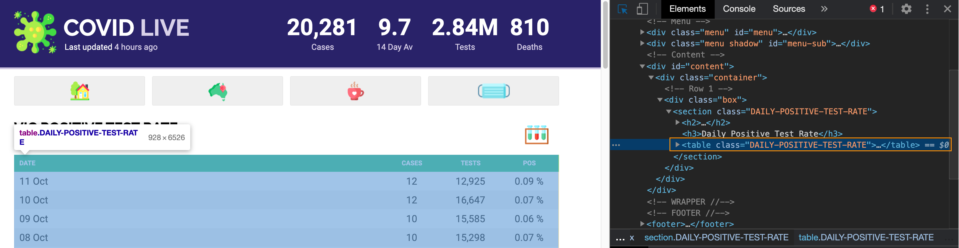
There are many ways to extract the right part of the site, but I like to just try getting the HTML table out using html_table(). We’re going to look at the output using str(), which provides a summary of the structure of the data to save ourselves printing all the HTML tables
bow(vic_test_url) %>%
  scrape() %>%
  html_table() %>%
  str()

#> List of 2
#>  $ :'data.frame':  2 obs. of  5 variables:
#>   ..$ X1: chr [1:2] "COVID LIVE" "Last updated 5 hours ago"
#>   ..$ X2: chr [1:2] "20,281" "Cases"
#>   ..$ X3: chr [1:2] "9.7" "14 Day Av"
#>   ..$ X4: chr [1:2] "2.84M" "Tests"
#>   ..$ X5: chr [1:2] "810" "Deaths"
#>  $ :'data.frame':  203 obs. of  4 variables:
#>   ..$ DATE : chr [1:203] "11 Oct" "10 Oct" "09 Oct" "08 Oct" ...
#>   ..$ CASES: int [1:203] 12 12 10 10 4 13 11 12 6 8 ...
#>   ..$ TESTS: chr [1:203] "12,925" "16,647" "15,585" "15,298" ...
#>   ..$ POS  : chr [1:203] "0.09 %" "0.07 %" "0.06 %" "0.07 %" ...
This tells us we want the second list element, which is the data frame, and then make that a tibble for nice printing:
bow(vic_test_url) %>%
  scrape() %>%
  html_table() %>%
  pluck(2) %>%
  as_tibble()

#> # A tibble: 203 x 4
#>    DATE   CASES TESTS  POS
#>    <chr>  <int> <chr>  <chr>
#>  1 11 Oct    12 12,925 0.09 %
#>  2 10 Oct    12 16,647 0.07 %
#>  3 09 Oct    10 15,585 0.06 %
#>  4 08 Oct    10 15,298 0.07 %
#>  5 07 Oct     4 16,429 0.02 %
#>  6 06 Oct    13 9,286  0.14 %
#>  7 05 Oct    11 9,023  0.12 %
#>  8 04 Oct    12 11,994 0.10 %
#>  9 03 Oct     6 11,281 0.05 %
#> 10 02 Oct     8 12,550 0.06 %
#> # … with 193 more rows
All together now:
vic_test_url <- "https://covidlive.com.au/report/daily-positive-test-rate/vic"

vic_test_data_raw <- bow(vic_test_url) %>%
  scrape() %>%
  html_table() %>%
  purrr::pluck(2) %>%
  as_tibble()

vic_test_data_raw

#> # A tibble: 203 x 4
#>    DATE   CASES TESTS  POS
#>    <chr>  <int> <chr>  <chr>
#>  1 11 Oct    12 12,925 0.09 %
#>  2 10 Oct    12 16,647 0.07 %
#>  3 09 Oct    10 15,585 0.06 %
#>  4 08 Oct    10 15,298 0.07 %
#>  5 07 Oct     4 16,429 0.02 %
#>  6 06 Oct    13 9,286  0.14 %
#>  7 05 Oct    11 9,023  0.12 %
#>  8 04 Oct    12 11,994 0.10 %
#>  9 03 Oct     6 11,281 0.05 %
#> 10 02 Oct     8 12,550 0.06 %
#> # … with 193 more rows
OK awesome, now let’s format the dates. We’ve got them in the format of the Day of the month in decimal form and then the 3 letter month abbreviation. We can convert this into a nice date object using strptime. This is a function I always forget how to use, so I end up browsing the help file every time and playing with a toy example until I get what I want. There are probably better ways, but this seems to work for me.
What this says is:
strptime("05 Oct", format = "%d %b")

#> [1] "2020-10-05 AEDT"
- Take the string, “05 Oct”
- The format that this follows is
- Day of the month as decimal number (01–31) (represented as “%d”)
- followed by a space, then
- Abbreviated month name in the current locale on this platform. (Also matches full name on input: in some locales there are no abbreviations of names.) (represented as “%d”).
For this to work, we need the string in the format argument to match EXACTLY the input. For example:
strptime("05-Oct", format = "%d %b")

#> [1] NA
Doesn’t work (because the dash)
But this:
strptime("05-Oct", format = "%d-%b")

#> [1] "2020-10-05 AEDT"
Does work, because the dash is in the format srtring.
OK and we want that as a Date object:
Let’s wrap this in a little function we can use on our data:
And double check it works:
strp_date("05 Oct")

#> [1] "2020-10-05"

strp_date("05 Oct") %>% class()

#> [1] "Date"
Ugh, dates.
OK, so now let’s clean up the dates.
vic_test_data_raw %>%
  mutate(DATE = strp_date(DATE))

#> # A tibble: 203 x 4
#>    DATE       CASES TESTS  POS
#>    <date>     <int> <chr>  <chr>
#>  1 2020-10-11    12 12,925 0.09 %
#>  2 2020-10-10    12 16,647 0.07 %
#>  3 2020-10-09    10 15,585 0.06 %
#>  4 2020-10-08    10 15,298 0.07 %
#>  5 2020-10-07     4 16,429 0.02 %
#>  6 2020-10-06    13 9,286  0.14 %
#>  7 2020-10-05    11 9,023  0.12 %
#>  8 2020-10-04    12 11,994 0.10 %
#>  9 2020-10-03     6 11,281 0.05 %
#> 10 2020-10-02     8 12,550 0.06 %
#> # … with 193 more rows
And let’s use parse_number to convert TESTS and POS into numbers, as they have commas in them and % signs, so R registers them as character strings.
vic_test_data_raw %>%
  mutate(DATE = strp_date(DATE),
         TESTS = parse_number(TESTS),
         POS = parse_number(POS))

#> # A tibble: 203 x 4
#>    DATE       CASES TESTS   POS
#>    <date>     <int> <dbl> <dbl>
#>  1 2020-10-11    12 12925  0.09
#>  2 2020-10-10    12 16647  0.07
#>  3 2020-10-09    10 15585  0.06
#>  4 2020-10-08    10 15298  0.07
#>  5 2020-10-07     4 16429  0.02
#>  6 2020-10-06    13  9286  0.14
#>  7 2020-10-05    11  9023  0.12
#>  8 2020-10-04    12 11994  0.1
#>  9 2020-10-03     6 11281  0.05
#> 10 2020-10-02     8 12550  0.06
#> # … with 193 more rows
parse_number() (from readr) is one of my favourite little functions, as this saves me a ton of effort.
Now let’s use clean_names() function from janitor to make the names all lower case, making them a bit nicer to deal with. (I don’t like holding down shift to type all caps for long periods of time, unless I’ve got something exciting to celebrate or scream).
vic_test_data_raw %>%
  mutate(DATE = strp_date(DATE),
         TESTS = parse_number(TESTS),
         POS = parse_number(POS)) %>%
  janitor::clean_names()

#> # A tibble: 203 x 4
#>    date       cases tests   pos
#>    <date>     <int> <dbl> <dbl>
#>  1 2020-10-11    12 12925  0.09
#>  2 2020-10-10    12 16647  0.07
#>  3 2020-10-09    10 15585  0.06
#>  4 2020-10-08    10 15298  0.07
#>  5 2020-10-07     4 16429  0.02
#>  6 2020-10-06    13  9286  0.14
#>  7 2020-10-05    11  9023  0.12
#>  8 2020-10-04    12 11994  0.1
#>  9 2020-10-03     6 11281  0.05
#> 10 2020-10-02     8 12550  0.06
#> # … with 193 more rows
And then finally all together now, I’m going to turn this into a tsibble - a time series tibble, using as_tsibble, and specifying the index (the time part) as the date column. I use this because later on we’ll be manipulating the date column, and tsibble makes this much easier.
library(tsibble)
vic_tests <- vic_test_data_raw %>%
  mutate(DATE = strp_date(DATE),
         TESTS = parse_number(TESTS),
         POS = parse_number(POS)) %>%
  janitor::clean_names() %>%
  rename(pos_pct = pos) %>%
  as_tsibble(index = date)
OK, now to iterate on a few plots.
ggplot(vic_tests,
         aes(x = date,
             y = pos_pct)) +
  geom_line()
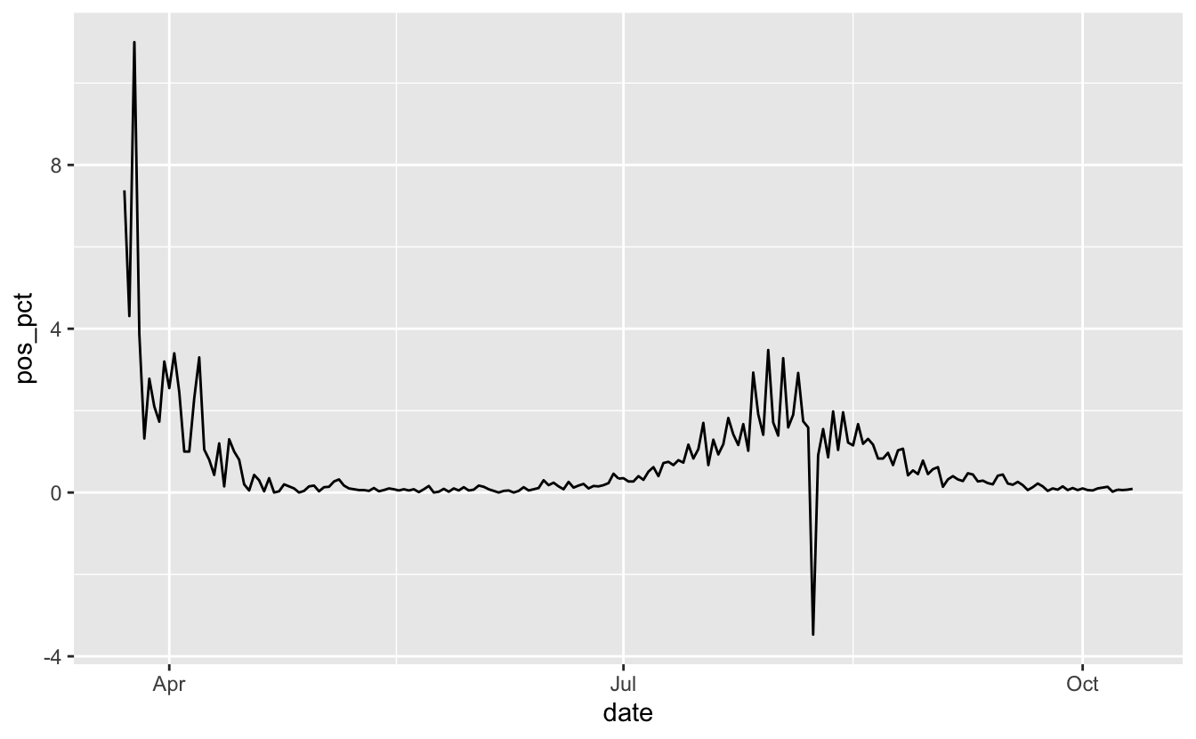
Oof, OK, let’s remove that negative date, not sure why that is there:
vic_tests_clean <- vic_tests %>%
  filter(pos_pct >= 0)

ggplot(vic_tests_clean,
         aes(x = date,
             y = pos_pct)) +
  geom_line()
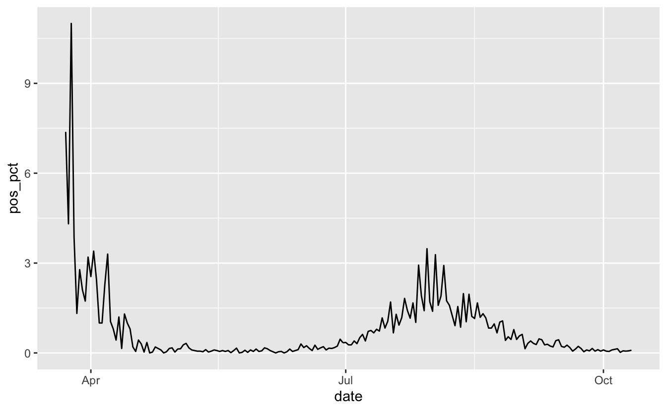
OK, looks like in April we have some high numbers, let’s bring filter out those dates from before May using filter_index - here we specify the start date, and the . means the last date:
vic_tests_clean %>%
  filter_index("2020-05-01" ~ .) %>%
  ggplot(aes(x = date,
             y = pos_pct)) +
  geom_line()
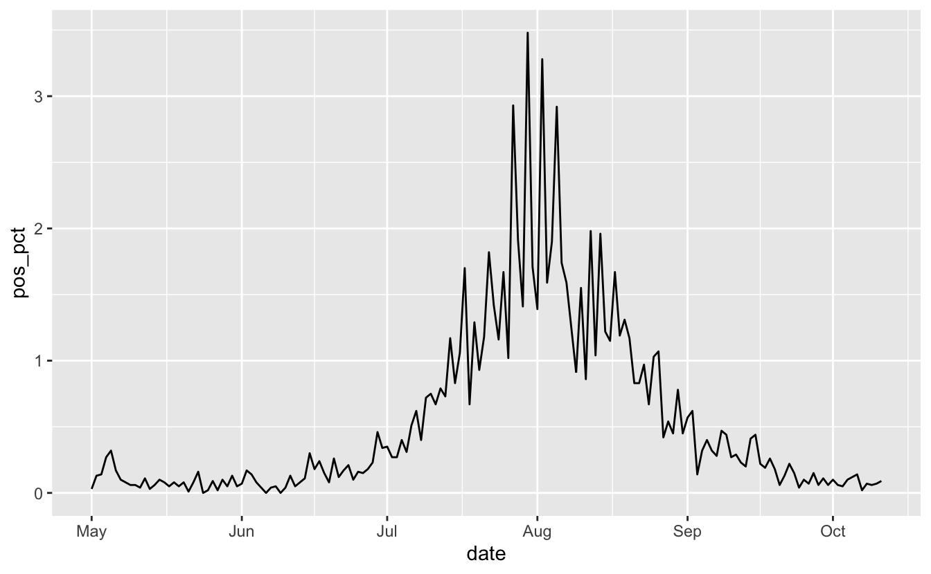
OK, much nicer. Looks like things are on the downward-ish. But the I want to add “%” signs to the plot. We could glue/paste those onto the data values, but I prefer to use the scales package for this part. We can browse the label_percent() reference page to see how to use it:
library(scales)
vic_tests_clean %>%
  filter_index("2020-05-01" ~ .) %>%
  ggplot(aes(x = date,
             y = pos_pct)) +
  geom_line() +
  scale_y_continuous(labels = label_percent())
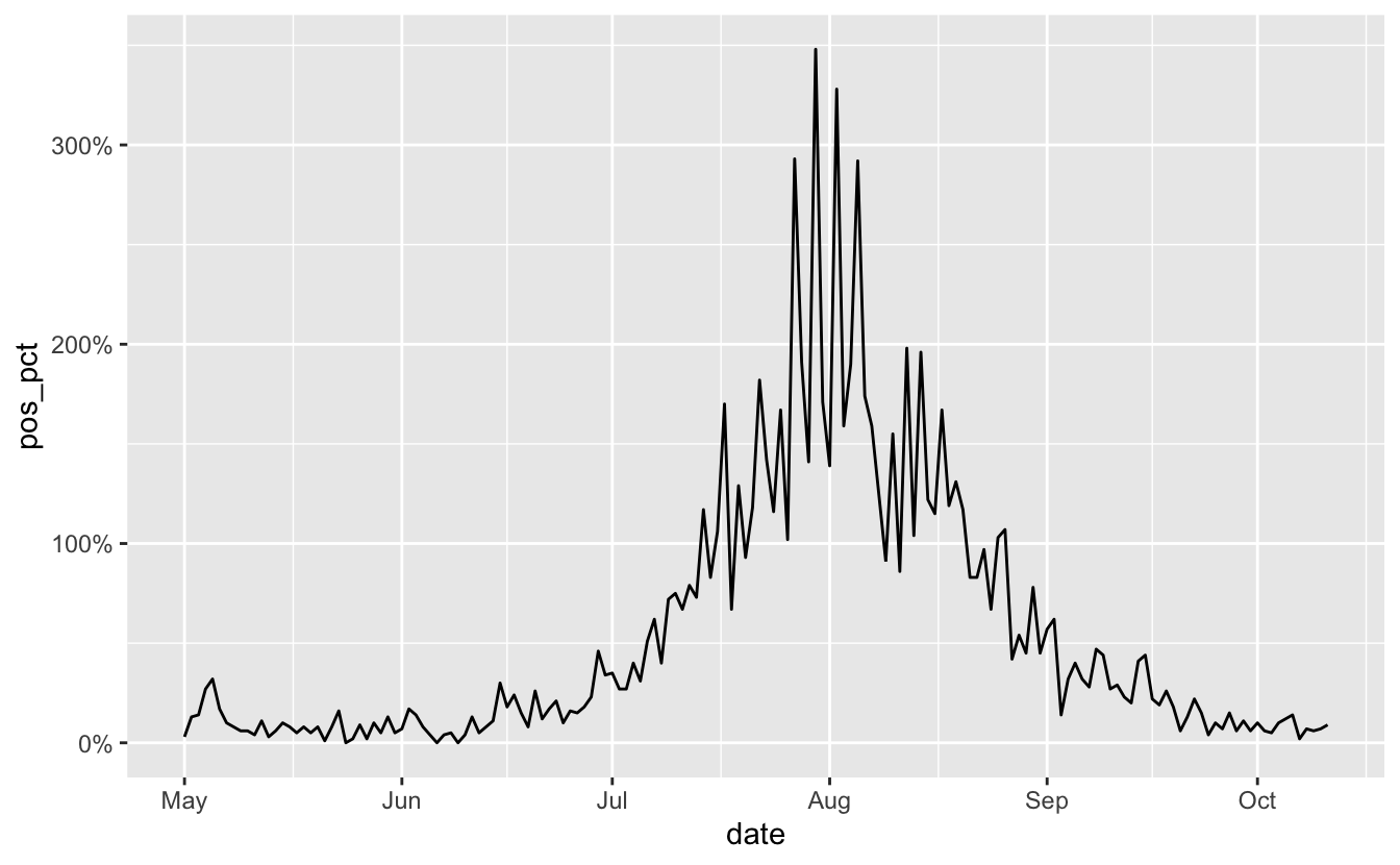
We specify how we want to change the y axis, using scale_y_continuous, and then say that the labels on the y axis need to have the label_percent function applied to them. Well, that’s how I read it.
OK, but this isn’t quite what we want actually, we need to change the scale - since by default it multiplies the number by 100. We also need to change the accuracy, since we want this to 2 decimal places. We can see this with the percent function, which is what label_percent uses under the hood.
percent(0.1)

#> [1] "10%"

percent(0.1, scale = 1)

#> [1] "0%"

percent(0.1, scale = 1, accuracy = 0.01)

#> [1] "0.10%"
So now we change the accuracy and scale arguments so we get the right looking marks.
library(scales)
vic_tests_clean %>%
  filter_index("2020-05-01" ~ .) %>%
  ggplot(aes(x = date,
             y = pos_pct)) +
  geom_line() +
  scale_y_continuous(labels = label_percent(accuracy = 0.01,
                                            scale = 1))
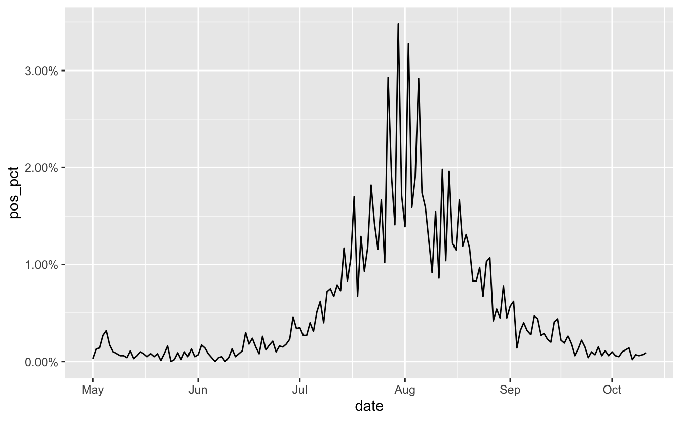
And that’s how to scrape some data, parse the dates, filter by time, and make the percentages print nice in a ggplot.
Thanks to Dmytro Perepolkin for polite, Earo Wang for tsibble, Sam Firke for janitor, the awesome tidyverse team for creating and maintaining the tidyverse, and of course the folks behind R, because R is great.