I’m please to say that visdat version 0.6.0 (codename: “Superman, Lazlo Bane”) is now on CRAN. This is the first release in nearly 3 years, there are a couple of new functions for visualising numeric and binary data, as well as some maintenance and bug fixes.
Let’s walk through some of the new features, bug fixes, and other misc changes.
New Features
vis_value() - visualise values
The idea of vis_value() is to visualise numeric data, so that you can get a quick idea of the values in your dataset. It does this by scaling all the data between 0 and 1, but it only works with numeric data.
vis_value(mtcars)
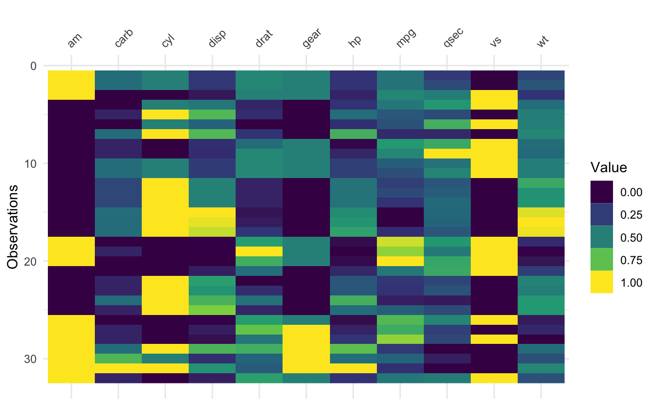
It can be fun and interesting to arrange by a variable and then show see how that changes the plot.
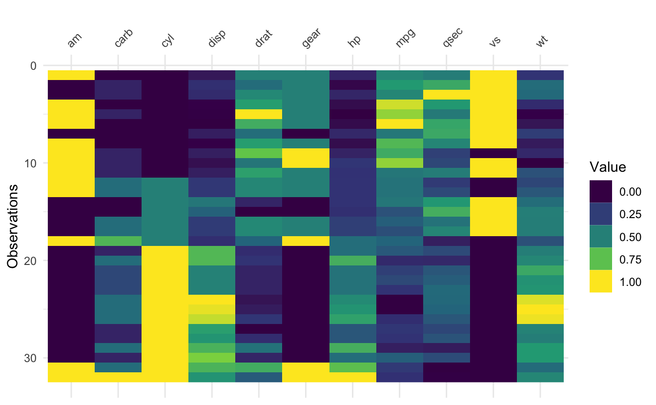
Although fair warning that there’s a whole set of statistics/data visualisation that focusses on how to arrange rows and columns - a technique called seriation. For a fun introduction, I’d recommend this lovely blogpost by Nicholas Kruchten. One day I will implement seriation in visdat.
Note that if you use vis_value() on a dataset that isn’t entirely numeric, you will get an error:
vis_value(diamonds)
#> Error in `test_if_all_numeric()` at visdat/R/vis-value.R:33:2:
#> ! Data input can only contain numeric values
#> Please subset the data to the numeric values you would like.
#> `dplyr::select(<data>, where(is.numeric))`
#> Can be helpful here!
vis_binary() visualise binary values
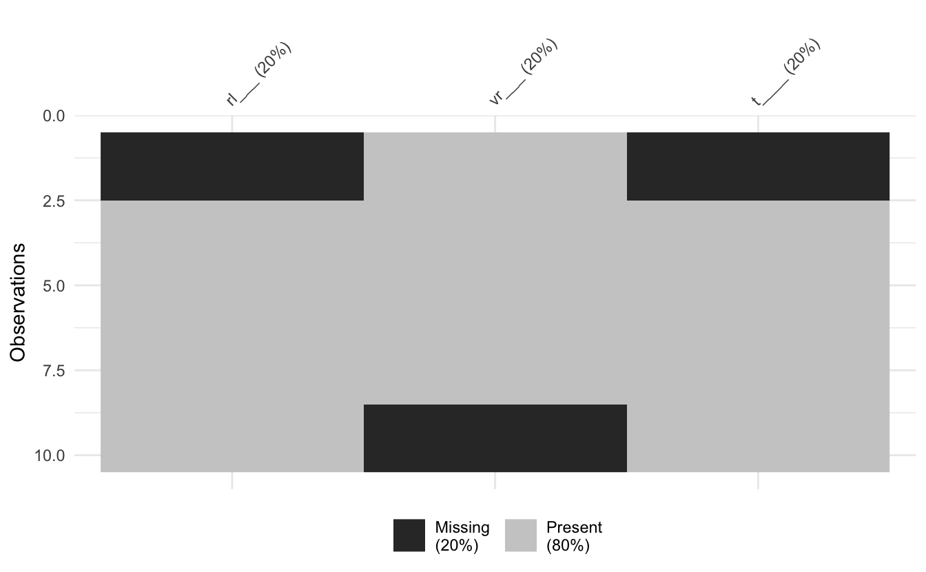
The vis_binary() function is for visualising datasets with binary values - similar to vis_value(), but just for binary data (0, 1, NA).
vis_binary(dat_bin)
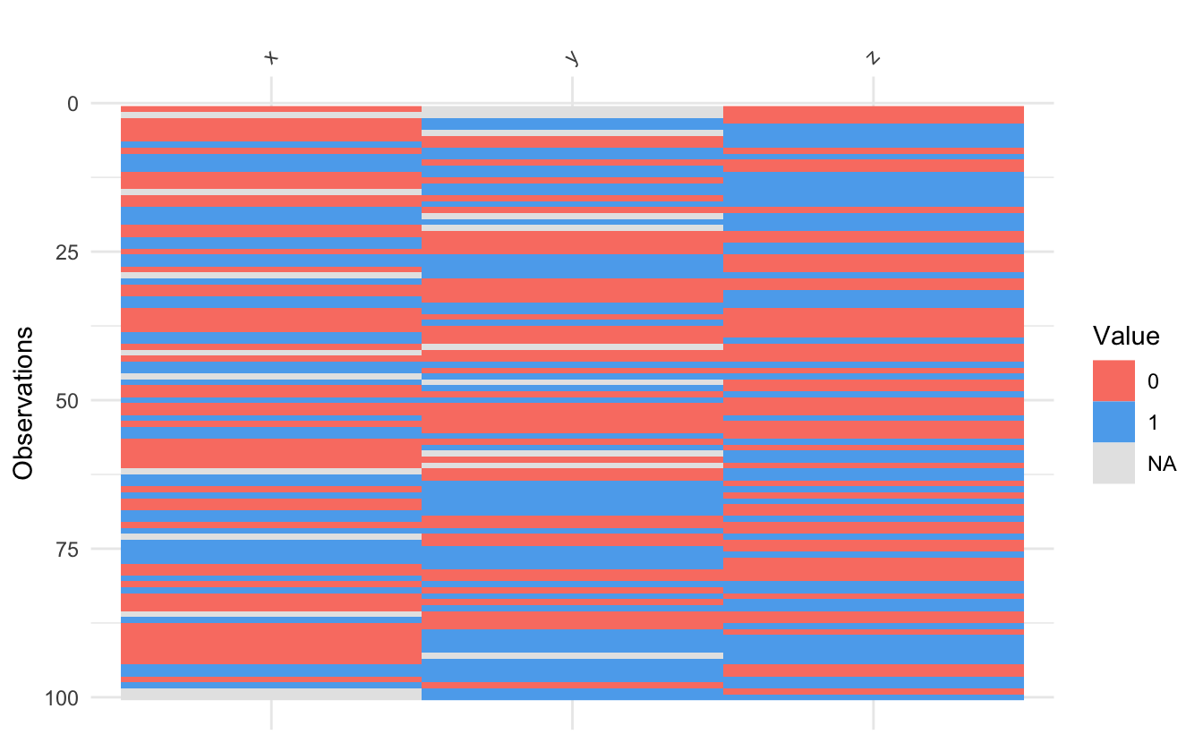
Thank you to Trish Gilholm for her suggested use case for this.
Facetting in visdat
It is now possible to perform facetting for the following functions in visdat: vis_dat(), vis_cor(), and vis_miss() via the facet argument. This lead to some internal cleaning up of package code (always fun to revisit some old code and refactor!) Here’s an example of facetting:
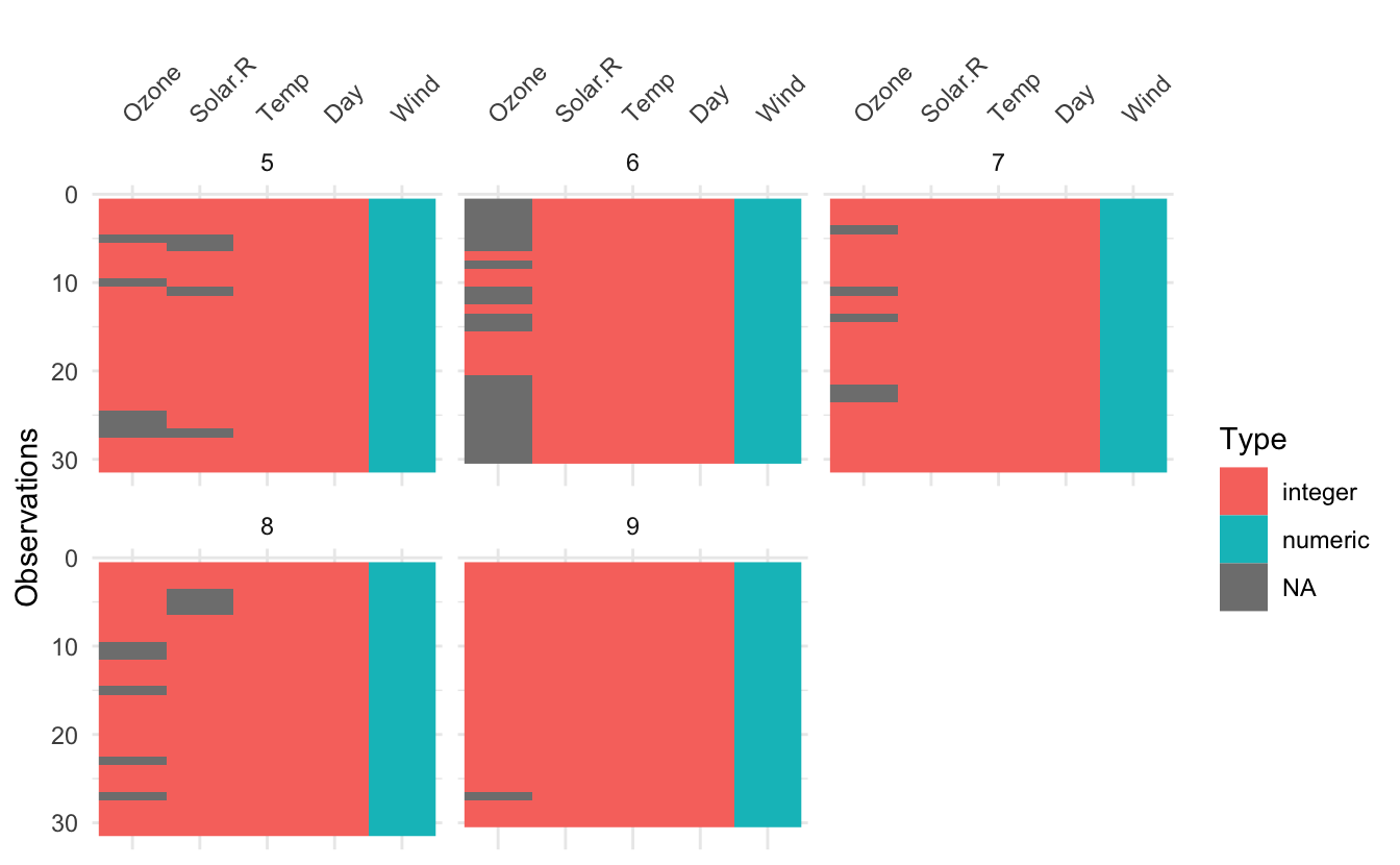
vis_dat(airquality, facet = Month)
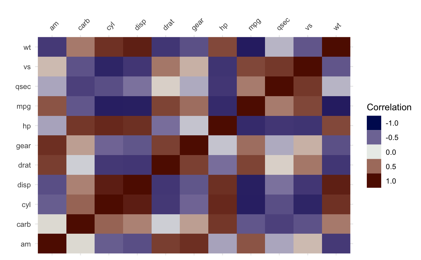
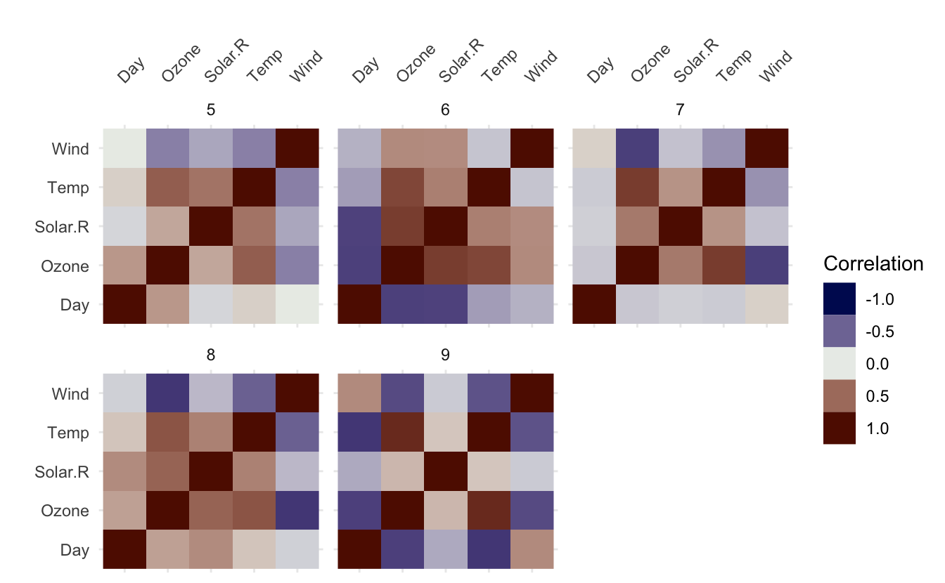
vis_cor(airquality, facet = Month)
vis_miss(airquality, facet = Month)
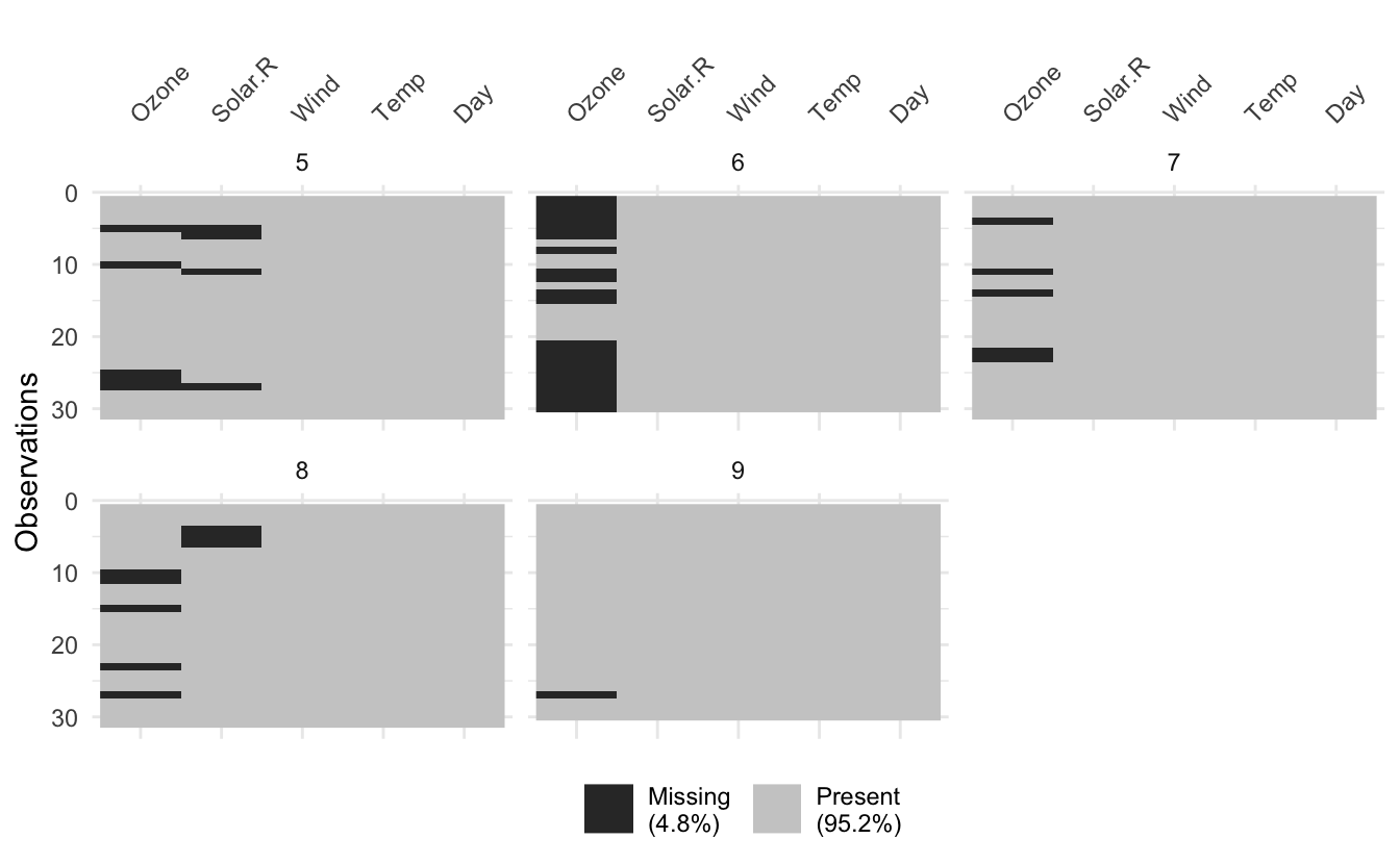
Notably for vis_miss when using facetting, you don’t get column missingness summaries, as I couldn’t quite work out how to do this for each facet.
Thank you to Sam Firke’s initial tweet on this that inspired this, and Jonathan Zadra’s contributions in the issue thread.
The next release will implement facetting for vis_value(), vis_binary(), vis_compare(), vis_expect(), and vis_guess() - see #159 to keep track.
Data methods for plotting
Related to facetting, I have implemented methods that provide data methods for plots with data_vis_dat(), data_vis_cor(), and data_vis_miss():
data_vis_dat(airquality)
#> # A tibble: 918 × 4
#>     rows variable valueType value
#>    <int> <chr>    <chr>     <chr>
#>  1     1 Day      integer   41
#>  2     1 Month    integer   190
#>  3     1 Ozone    integer   7.4
#>  4     1 Solar.R  integer   67
#>  5     1 Temp     integer   5
#>  6     1 Wind     numeric   1
#>  7     2 Day      integer   36
#>  8     2 Month    integer   118
#>  9     2 Ozone    integer   8
#> 10     2 Solar.R  integer   72
#> # … with 908 more rows
data_vis_miss(airquality)
#> # A tibble: 918 × 4
#>     rows variable valueType value
#>    <int> <chr>    <chr>     <chr>
#>  1     1 Day      FALSE     FALSE
#>  2     1 Month    FALSE     FALSE
#>  3     1 Ozone    FALSE     FALSE
#>  4     1 Solar.R  FALSE     FALSE
#>  5     1 Temp     FALSE     FALSE
#>  6     1 Wind     FALSE     FALSE
#>  7     2 Day      FALSE     FALSE
#>  8     2 Month    FALSE     FALSE
#>  9     2 Ozone    FALSE     FALSE
#> 10     2 Solar.R  FALSE     FALSE
#> # … with 908 more rows
data_vis_cor(airquality)
#> # A tibble: 36 × 3
#>    row_1   row_2     value
#>    <chr>   <chr>     <dbl>
#>  1 Ozone   Ozone    1
#>  2 Ozone   Solar.R  0.348
#>  3 Ozone   Wind    -0.602
#>  4 Ozone   Temp     0.698
#>  5 Ozone   Month    0.165
#>  6 Ozone   Day     -0.0132
#>  7 Solar.R Ozone    0.348
#>  8 Solar.R Solar.R  1
#>  9 Solar.R Wind    -0.0568
#> 10 Solar.R Temp     0.276
#> # … with 26 more rows
The implementation of this works by providing these functions as S3 methods that have a .grouped_df method to facilitate plotting with facets.
airquality %>% group_by(Month) %>% data_vis_dat()
#> # A tibble: 765 × 5
#> # Groups:   Month [5]
#>    Month  rows variable valueType value
#>    <int> <int> <chr>    <chr>     <chr>
#>  1     5     1 Day      integer   41
#>  2     5     1 Ozone    integer   190
#>  3     5     1 Solar.R  integer   7.4
#>  4     5     1 Temp     integer   67
#>  5     5     1 Wind     numeric   1
#>  6     5     2 Day      integer   36
#>  7     5     2 Ozone    integer   118
#>  8     5     2 Solar.R  integer   8
#>  9     5     2 Temp     integer   72
#> 10     5     2 Wind     numeric   2
#> # … with 755 more rows
Missing values show up in list columns
vis_dat() vis_miss() and vis_guess() now render missing values in list-columns. Let’s demonstrate this with the star_wars dataset from dplyr, which has a few list columns.
starwars
#> # A tibble: 87 × 14
#> name height mass hair_…¹ skin_…² eye_c…³ birth…⁴ sex gender homew…⁵
#> <chr> <int> <dbl> <chr> <chr> <chr> <dbl> <chr> <chr> <chr>
#> 1 Luke Skywa… 172 77 blond fair blue 19 male mascu… Tatooi…
#> 2 C-3PO 167 75 NA gold yellow 112 none mascu… Tatooi…
#> 3 R2-D2 96 32 NA white,… red 33 none mascu… Naboo
#> 4 Darth Vader 202 136 none white yellow 41.9 male mascu… Tatooi…
#> 5 Leia Organa 150 49 brown light brown 19 fema… femin… Aldera…
#> 6 Owen Lars 178 120 brown,… light blue 52 male mascu… Tatooi…
#> 7 Beru White… 165 75 brown light blue 47 fema… femin… Tatooi…
#> 8 R5-D4 97 32 NA white,… red NA none mascu… Tatooi…
#> 9 Biggs Dark… 183 84 black light brown 24 male mascu… Tatooi…
#> 10 Obi-Wan Ke… 182 77 auburn… fair blue-g… 57 male mascu… Stewjon
#> # … with 77 more rows, 4 more variables: species <chr>, films <list>,
#> # vehicles <list>, starships <list>, and abbreviated variable names
#> # ¹hair_color, ²skin_color, ³eye_color, ⁴birth_year, ⁵homeworld
glimpse(starwars)
#> Rows: 87
#> Columns: 14
#> $ name       <chr> "Luke Skywalker", "C-3PO", "R2-D2", "Darth Vader", "Leia Or…
#> $ height     <int> 172, 167, 96, 202, 150, 178, 165, 97, 183, 182, 188, 180, 2…
#> $ mass       <dbl> 77.0, 75.0, 32.0, 136.0, 49.0, 120.0, 75.0, 32.0, 84.0, 77.…
#> $ hair_color <chr> "blond", NA, NA, "none", "brown", "brown, grey", "brown", N…
#> $ skin_color <chr> "fair", "gold", "white, blue", "white", "light", "light", "…
#> $ eye_color  <chr> "blue", "yellow", "red", "yellow", "brown", "blue", "blue",…
#> $ birth_year <dbl> 19.0, 112.0, 33.0, 41.9, 19.0, 52.0, 47.0, NA, 24.0, 57.0, …
#> $ sex        <chr> "male", "none", "none", "male", "female", "male", "female",…
#> $ gender     <chr> "masculine", "masculine", "masculine", "masculine", "femini…
#> $ homeworld  <chr> "Tatooine", "Tatooine", "Naboo", "Tatooine", "Alderaan", "T…
#> $ species    <chr> "Human", "Droid", "Droid", "Human", "Human", "Human", "Huma…
#> $ films      <list> <"The Empire Strikes Back", "Revenge of the Sith", "Return…
#> $ vehicles   <list> <"Snowspeeder", "Imperial Speeder Bike">, <>, <>, <>, "Imp…
#> $ starships  <list> <"X-wing", "Imperial shuttle">, <>, <>, "TIE Advanced x1",…
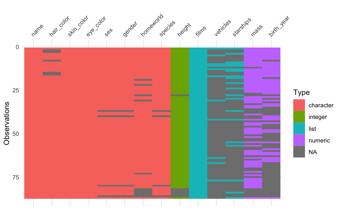
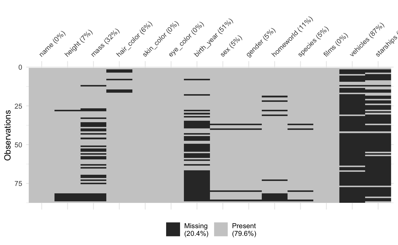
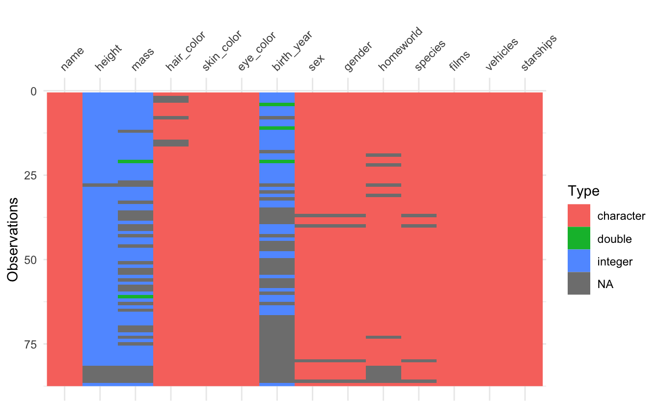
As you can see, lists are now displayed in the visualisation. Unfortunately vis_guess has trouble guessing lists, but that is a limitation due to how it guesses variable types.
Thank you to github user cregouby for adding this in #138.
Abbreviation helpers
Long variable names can be annoying and can crowd a plot. The abbreviate_vars() function can be used to help with this:
long_data <- tibble(
  really_really_long_name = c(NA, NA, 1:8),
  very_quite_long_name = c(-1:-8, NA, NA),
  this_long_name_is_something_else = c(NA, NA,
                                       seq(from = 0, to = 1, length.out = 8))
)

vis_miss(long_data)
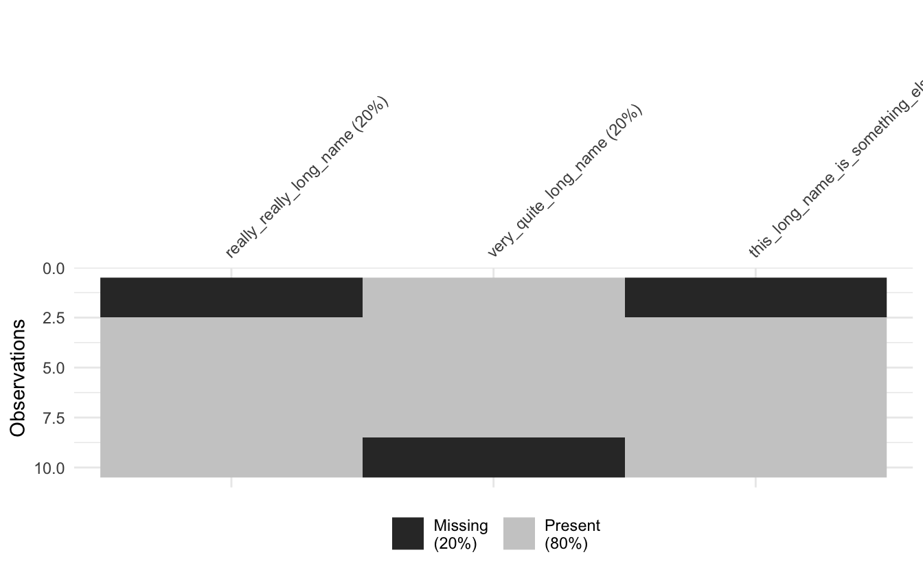
Ugh no good.
Use abbreviate_vars() to help:
long_data %>% abbreviate_vars() %>% vis_miss()
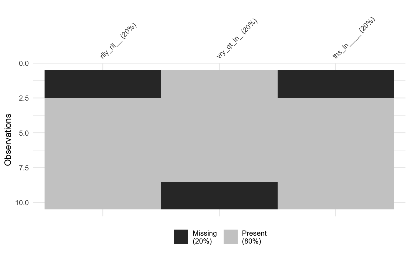
You can control the length of the abbreviation with min_length:
long_data %>% abbreviate_vars(min_length = 5) %>% vis_miss()
Under the hood this uses the base R function, abbreviate() - a gem of a function.
Thank you to chapau3, and ivanhanigan for requesting this feature (#140 and #9).
Missingness percentages are now integers.
The vis_miss() function shows a percentage missing of the missing values in each column - I’ve decided to make this round to integers, as it is only a guide and I found them to be a bit cluttered. I also do not like the idea of extracting summary statistics from graphics, so they now look like this:
vis_miss(airquality)
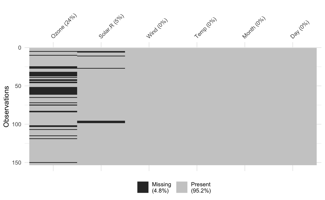
For more accurate representation of missingness summaries please use the naniar R package functions like miss_var_summary():
library(naniar)
miss_var_summary(airquality)
#> # A tibble: 6 × 3
#>   variable n_miss pct_miss
#>   <chr>     <int>    <dbl>
#> 1 Ozone        37    24.2
#> 2 Solar.R       7     4.58
#> 3 Wind          0     0
#> 4 Temp          0     0
#> 5 Month         0     0
#> 6 Day           0     0
Which also works with dplyr::group_by():
airquality %>%
  group_by(Month) %>%
  miss_var_summary()
#> # A tibble: 25 × 4
#> # Groups:   Month [5]
#>    Month variable n_miss pct_miss
#>    <int> <chr>     <int>    <dbl>
#>  1     5 Ozone         5     16.1
#>  2     5 Solar.R       4     12.9
#>  3     5 Wind          0      0
#>  4     5 Temp          0      0
#>  5     5 Day           0      0
#>  6     6 Ozone        21     70
#>  7     6 Solar.R       0      0
#>  8     6 Wind          0      0
#>  9     6 Temp          0      0
#> 10     6 Day           0      0
#> # … with 15 more rows
If you find that this really bothers you and you want to have control over the percentage missingness in the columns, please file an issue on visdat and I will look into adding more user control. Ideally I would have added control for users in the first place, but it just wasn’t something I was certain users wanted, and would require more arguments to a function, which require more tests…and so on. So with the mindset of keeping this package easy to maintain, I figured this might be the easiest way forward.
Bug Fixes and Other changes
Here is a quick listing of the other changes in this release of visdat:
- No longer use
gatherinternally: #141 - Resolve bug where
vis_value()displayed constant values as NA values 128 - these constant values are now shown as 1. - Removed use of the now deprecated “aes_string” from ggplot2
- Output of plot in
vis_expectwould reorder columns (#133), fixed in #143 by muschellij2. - A new vignette on customising colour palettes in visdat, “Customising colour palettes in visdat”.
- No longer uses gdtools for testing #145
- Use
cliinternally for error messages. - Speed up some internal functions
Thanks
Thank you to all the users who contributed to this release!