
Data packages are something that have been on my mind a bit lately, having recently worked on the ozroaddeaths data access package at the rOpenSci ozunconf. I was reading Joe Rickert’s R views blogpost about data packages in R, and saw the billboard package by Mikkel Krogsholm, which provides:
… data sets regarding songs on the Billboard Hot 100 list from 1960 to 2016, including ranks for the given year, musical features, and lyrics.
This seemed like a really cool dataset to look at, so last weekend I started to have a dig around and noticed that it had some nice examples of data munging with tidyverse packages and friends, and it seemed like it would make a nice blogpost case study, of sorts.
So, this blogpost walks through how you might start to unpack the data, clean it, and draw some interesting conclusions. I also wanted to avoid the “draw the rest of the fucking owl” problem.

This means that we don’t start with a perfectly clean dataset, and I try to take a bit of time to walk through some of the code.
So, first things first, we’re going to load up our packages:
billboardfor the data;tidyverse, to provide the nice tools we need to clean up and visualise the data;visdat, which helps assist in pre-exploratory data analysis.
library(billboard)
library(tidyverse)
## ── Attaching packages ────────────────────────────────────────────── tidyverse 1.2.1 ──
## ✔ ggplot2 2.2.1     ✔ purrr   0.2.4
## ✔ tibble  1.4.2     ✔ dplyr   0.7.4
## ✔ tidyr   0.8.0     ✔ stringr 1.2.0
## ✔ readr   1.1.1     ✔ forcats 0.2.0
## ── Conflicts ───────────────────────────────────────────────── tidyverse_conflicts() ──
## ✖ dplyr::filter() masks stats::filter()
## ✖ dplyr::lag()    masks stats::lag()
library(visdat)
Data Munging
According to the help file for wiki_hot_100s, this data contains:
57 years of Billboards Hot 100 songs. The data is scraped from Wikipedia from the urls ‘https://en.wikipedia.org/wiki/Billboard_Year-End_Hot_100_singles_of_' and then the year added. Example: https://en.wikipedia.org/wiki/Billboard_Year-End_Hot_100_singles_of_1960. One year has more than a 100 songs due to a tie.
It then states the following info about the variables:
A data frame with 5701 rows and 4 variables:
no: the rank that the song had that year
title: the title of the song
artist: the artist of the song
year: year
Before we go ahead and jump into analysing the data, it’s a good idea to do have a look at the data, with vis_dat.
vis_dat(wiki_hot_100s)
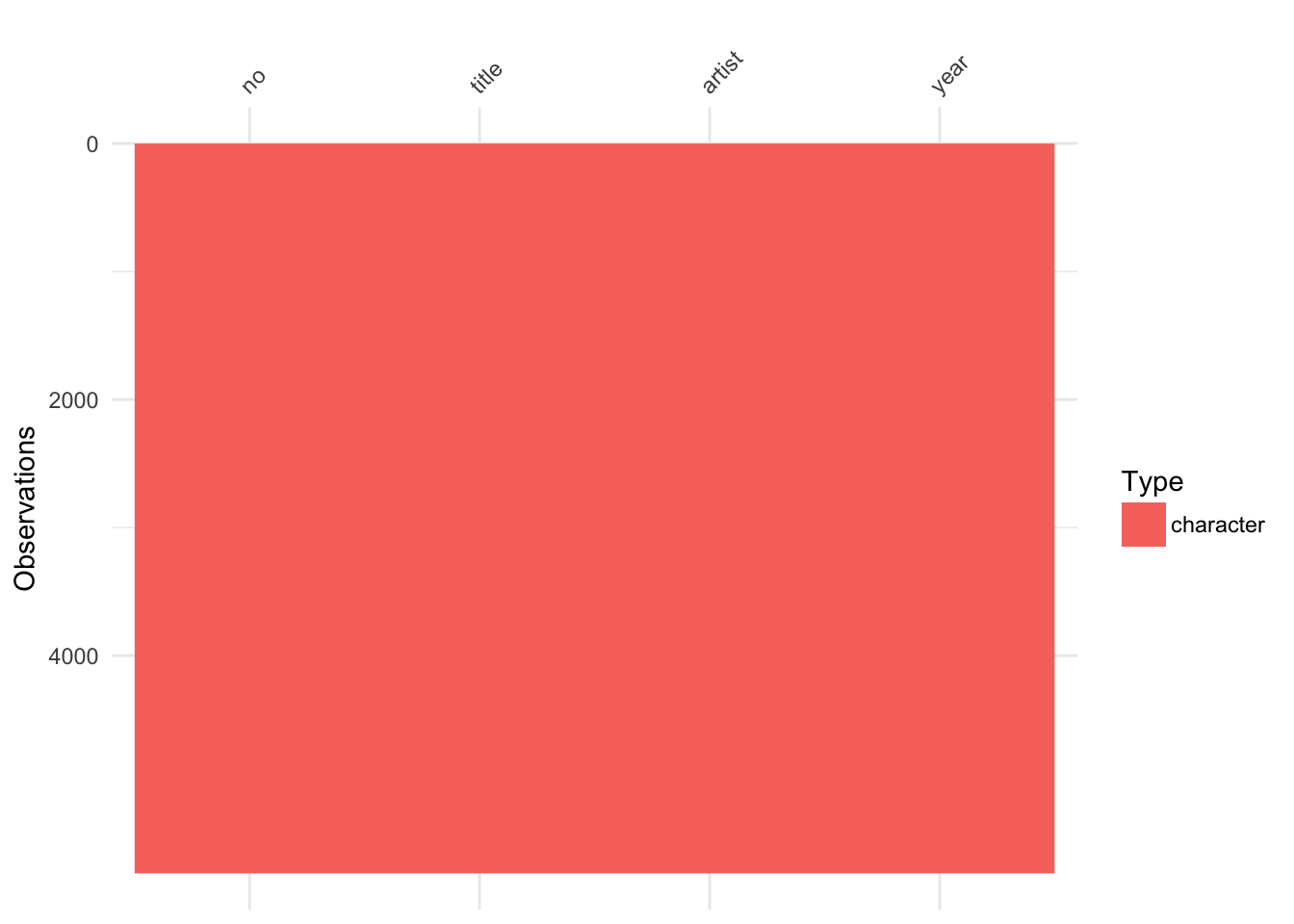
vis_dat gives you a birds eye view of the data, showing the class of each variable, and also displays missing data (if there is any). In this case, we can see that there is no missing data, and that everything is a character.
I would expect year and rank (marked as “no”) to be numbers, not characters, so let’s have a closer look at these.
But first, let’s convert it to a tibble, which, among other things, is basically the same as a normal data.frame, but gives a nice print method, so it only shows the first 10 rows by default, and gives some text describing the data type.
billboard_raw <- as_tibble(wiki_hot_100s)
billboard_raw
## # A tibble: 5,701 x 4
##    no    title                     artist              year
##    <chr> <chr>                     <chr>               <chr>
##  1 1     Theme from A Summer Place Percy Faith         1960
##  2 2     He'll Have to Go          Jim Reeves          1960
##  3 3     Cathy's Clown             The Everly Brothers 1960
##  4 4     Running Bear              Johnny Preston      1960
##  5 5     Teen Angel                Mark Dinning        1960
##  6 6     I'm Sorry                 Brenda Lee          1960
##  7 7     It's Now or Never         Elvis Presley       1960
##  8 8     Handy Man                 Jimmy Jones         1960
##  9 9     Stuck on You              Elvis Presley       1960
## 10 10    The Twist                 Chubby Checker      1960
## # ... with 5,691 more rows
This is nice because it means you don’t have to consciously think about what might happen when you want to view the data - it doesn’t just vomit out the ENTIRE dataframe when you type wiki_hot_100s.
OK, so we can see that no and year are characters, but really they should be numeric, as they aren’t written as “Number One” and “Nineteen Sixty”, so let’s coerce them into numbers with as.numeric. We also create another variable, rank, which is a more descriptive word than no.
billboard_raw %>%
  mutate(rank = as.numeric(no),
         year = as.numeric(year))
## Warning in evalq(as.numeric(no), <environment>): NAs introduced by coercion
## # A tibble: 5,701 x 5
##    no    title                     artist               year  rank
##    <chr> <chr>                     <chr>               <dbl> <dbl>
##  1 1     Theme from A Summer Place Percy Faith          1960  1.00
##  2 2     He'll Have to Go          Jim Reeves           1960  2.00
##  3 3     Cathy's Clown             The Everly Brothers  1960  3.00
##  4 4     Running Bear              Johnny Preston       1960  4.00
##  5 5     Teen Angel                Mark Dinning         1960  5.00
##  6 6     I'm Sorry                 Brenda Lee           1960  6.00
##  7 7     It's Now or Never         Elvis Presley        1960  7.00
##  8 8     Handy Man                 Jimmy Jones          1960  8.00
##  9 9     Stuck on You              Elvis Presley        1960  9.00
## 10 10    The Twist                 Chubby Checker       1960 10.0
## # ... with 5,691 more rows
This gives us a warning - “NAs introduced by coercion”. This tells us something went wrong. Let’s see where those values are NA, and what’s going on there by filtering our observations to see only those that are missing using filter(is.na(rank)).
billboard_raw %>%
  mutate(rank = as.numeric(no),
         year = as.numeric(year)) %>%
  filter(is.na(rank))
## Warning in evalq(as.numeric(no), <environment>): NAs introduced by coercion
## # A tibble: 5 x 5
##   no    title                          artist                   year  rank
##   <chr> <chr>                          <chr>                   <dbl> <dbl>
## 1 Tie   Let Me                         Paul Revere & the Raid…  1969    NA
## 2 Tie   Rock Your Baby                 George McCrae            1974    NA
## 3 Tie   Never, Never Gonna Give You Up Barry White              1974    NA
## 4 Tie   The Lord's Prayer              Sister Janet Mead        1974    NA
## 5 Tie   My Mistake (Was to Love You)   Diana Ross & Marvin Ga…  1974    NA
Huh, turns out that “Tie” is a category for 1974 and 1969, this was mentioned in the description of the data in the help file, but I just assumed that they would be given the same rank.
Now, we could look at the surrounding rows of the “Tie” columns more closely by simply filtering according to those years, 1969 and 1974, and using View().

BUT, if you had like a thousand, or say, one bajillion rows to look at then this doesn’t really work.
So instead we are going to find the row numbers where this occurs, and then look at them.
We do this by first creating a new variable containing the row numbers (1 through to the number of rows in the dataset), then filter those observations that are marked as “Tie”, then pull out the row_numbers as a vector with the relatively new pull function, which returns the values from a dataframe as a vector, rather than a smaller dataframe, which you would get with select.
row_tie <- billboard_raw %>%
  mutate(row_num = 1:n()) %>%
  filter(no == "Tie") %>%
  pull(row_num)

row_tie
## [1] 1001 1439 1456 1487 1493
These row locations, 1001, 1439, 1456, 1487, 1493, are where these tie’s occur.
What we want to do now is look at the rows before and after these ones with the tie, to get a sense of what rank these Tied values have. You can think of this as padding out the rows around it. We can pad out the numbers by adding one and subtracting one, to get the rows around the tied rows, and then sort them, to give the row numbers with the ties plus the previous and subsequent rows.
row_pad <- c(row_tie,
             row_tie + 1,
             row_tie -1) %>%
  sort()

row_pad
##  [1] 1000 1001 1002 1438 1439 1440 1455 1456 1457 1486 1487 1488 1492 1493
## [15] 1494
Finally, you can then use this new vector and tell dplyr to display the slice of rows containing those numbers:
billboard_raw %>% slice(row_pad)
## # A tibble: 15 x 4
##    no    title                                 artist                year
##    <chr> <chr>                                 <chr>                 <chr>
##  1 100   Sweet Cream Ladies                    The Box Tops          1969
##  2 Tie   Let Me                                Paul Revere & the Ra… 1969
##  3 1     Bridge over Troubled Water            Simon & Garfunkel     1970
##  4 37    Nothing from Nothing                  Billy Preston         1974
##  5 Tie   Rock Your Baby                        George McCrae         1974
##  6 39    Top of the World                      The Carpenters        1974
##  7 54    You Won't See Me                      Anne Murray           1974
##  8 Tie   Never, Never Gonna Give You Up        Barry White           1974
##  9 56    Tell Me Something Good                Rufus & Chaka Khan    1974
## 10 85    I'll Have to Say I Love You in a Song Jim Croce             1974
## 11 Tie   The Lord's Prayer                     Sister Janet Mead     1974
## 12 87    Trying To Hold On To My Woman         Lamont Dozier         1974
## 13 91    Helen Wheels                          Paul McCartney and W… 1974
## 14 Tie   My Mistake (Was to Love You)          Diana Ross & Marvin … 1974
## 15 93    Wildwood Weed                         Jim Stafford          1974
What we see here is that a “Tie” takes on the value of the previous row. so we can now replace this with the value of the previous row, using the lag function, which turns a sequence like this:
x <- c(1,2,3)
Into this:
lag(x)
## [1] NA 1 2
billboard_raw %>%
  mutate(rank = as.numeric(no)) %>%
  mutate(rank_lag = lag(rank)) %>%
  select(no,rank,rank_lag) %>%
  mutate(rank_rep = if_else(is.na(rank),
                            true = rank_lag,
                            false = rank)) %>%
  filter(is.na(rank))
## Warning in evalq(as.numeric(no), <environment>): NAs introduced by coercion
## # A tibble: 5 x 4
##   no     rank rank_lag rank_rep
##   <chr> <dbl>    <dbl>    <dbl>
## 1 Tie      NA    100      100
## 2 Tie      NA     37.0     37.0
## 3 Tie      NA     54.0     54.0
## 4 Tie      NA     85.0     85.0
## 5 Tie      NA     91.0     91.0
OK, now let’s quickly check what these values are:
billboard_raw %>%
  mutate(rank = as.numeric(no)) %>%
  mutate(rank_lag = lag(rank)) %>%
  select(no,rank,rank_lag) %>%
  mutate(rank_rep = if_else(is.na(rank),
                            true = rank_lag,
                            false = rank)) %>%
  slice(row_pad)
## Warning in evalq(as.numeric(no), <environment>): NAs introduced by coercion
## # A tibble: 15 x 4
##    no      rank rank_lag rank_rep
##    <chr>  <dbl>    <dbl>    <dbl>
##  1 100   100        99.0   100
##  2 Tie    NA       100     100
##  3 1       1.00     NA       1.00
##  4 37     37.0      36.0    37.0
##  5 Tie    NA        37.0    37.0
##  6 39     39.0      NA      39.0
##  7 54     54.0      53.0    54.0
##  8 Tie    NA        54.0    54.0
##  9 56     56.0      NA      56.0
## 10 85     85.0      84.0    85.0
## 11 Tie    NA        85.0    85.0
## 12 87     87.0      NA      87.0
## 13 91     91.0      90.0    91.0
## 14 Tie    NA        91.0    91.0
## 15 93     93.0      NA      93.0
OK great, so now we can combine all of these steps (also renaming the column no to be rank). This is our clean data, so we call it billboard_clean.
billboard_clean <- billboard_raw %>%
  mutate(rank = as.numeric(no),
         year = as.numeric(year),
         rank_lag = lag(rank),
         rank_rep = if_else(condition = is.na(rank),
                            true = rank_lag,
                            false = rank)) %>%
  select(rank_rep,
         title,
         artist,
         year) %>%
  rename(rank = rank_rep)
## Warning in evalq(as.numeric(no), <environment>): NAs introduced by coercion
Note: This is a common pattern that I like to use - build up chains of commands with the
magrittrpipe operator until you are confident that they work. Then, you combine them together to create an object. This saves you creating intermediate objects like “data_1”, “data_check_lag”, “data_insert_lag_lead”, etc.
So now we’ve got a clean dataset, let’s think about something interesting to look at in this cool dataset!
One hit wonders
Let’s look at the one hit wonders in this list.
We first add the count, which creates a count of the number of times that each artist appears, and adds it back onto the dataset as a column. It saves doing some fandangling with joins, and was suggested by David Robinson in yet another awesome Rstats moment / design decision being made on twitter.
billboard_clean %>%
  add_count(artist)
## # A tibble: 5,701 x 5
##     rank title                     artist               year     n
##    <dbl> <chr>                     <chr>               <dbl> <int>
##  1  1.00 Theme from A Summer Place Percy Faith          1960     1
##  2  2.00 He'll Have to Go          Jim Reeves           1960     1
##  3  3.00 Cathy's Clown             The Everly Brothers  1960     6
##  4  4.00 Running Bear              Johnny Preston       1960     2
##  5  5.00 Teen Angel                Mark Dinning         1960     1
##  6  6.00 I'm Sorry                 Brenda Lee           1960    11
##  7  7.00 It's Now or Never         Elvis Presley        1960    16
##  8  8.00 Handy Man                 Jimmy Jones          1960     2
##  9  9.00 Stuck on You              Elvis Presley        1960    16
## 10 10.0  The Twist                 Chubby Checker       1960     5
## # ... with 5,691 more rows
What we then want to do is see how many bands have the rank of 1 and have only appeared once (n = 1).
# What about one hit wonders?

billboard_clean %>%
  add_count(artist) %>%
  filter(rank == 1, n == 1)
## # A tibble: 15 x 5
##     rank title                        artist                    year     n
##    <dbl> <chr>                        <chr>                    <dbl> <int>
##  1  1.00 Theme from A Summer Place    Percy Faith               1960     1
##  2  1.00 Stranger on the Shore        Acker Bilk                1962     1
##  3  1.00 Ballad of the Green Berets   SSgt. Barry Sadler        1966     1
##  4  1.00 To Sir With Love             Lulu                      1967     1
##  5  1.00 Sugar, Sugar                 The Archies               1969     1
##  6  1.00 My Sharona                   The Knack                 1979     1
##  7  1.00 Careless Whisper             Wham! featuring George …  1985     1
##  8  1.00 That's What Friends Are For  Dionne and Friends (Dio…  1986     1
##  9  1.00 Yeah!                        Usher featuring Lil Jon…  2004     1
## 10  1.00 Bad Day                      Daniel Powter             2006     1
## 11  1.00 Low                          Flo Rida featuring T-Pa…  2008     1
## 12  1.00 Somebody That I Used to Know Gotye featuring Kimbra    2012     1
## 13  1.00 Thrift Shop                  Macklemore and Ryan Lew…  2013     1
## 14  1.00 Happy                        Pharrell Williams         2014     1
## 15  1.00 Uptown Funk                  Mark Ronson featuring B…  2015     1
15 songs!
I would have thought more.
Alright, some interesting ones here. Some personal favourites include:
- Sugar, Sugar, by The Archies
- My Sharona, by The Knack (do yourself a favour and listent to the insane guitar solo at 2:45, seriously, how did this band not make it?)
- Careless Whisper, by Wham! Feat. George Michael
I’ve actually turned these into a public spotify playlist if you want to listen to them - it’s interesting to track the progress over time of these songs.
Of course, there are a few problems with this - there are a few artists on there who do special duets and “one offs”, like “Dionne and Friends”, which is made up of Dionne Warwick, Elton John, Gladys Knight, and Stevie Wonder, three of who have many hits. Also, some of these artists are more likely to enter the list again, for example, it wouldn’t surprise me if Macklemore, Pharrell, and Mark Ronson make it in again in the future. So while they are currently one hit wonders, it doesn’t mean that they won’t have another hit.
Hmm, on that note, what is the spread of years between entering the list twice or more? Let’s calculate the distance from the latest year to the earliest year for each artist, and look at those who have had a “long reign”, say more than 10 years.
billboard_clean %>%
  group_by(artist) %>%
  summarise(year_dist = max(year) - min(year)) %>%
  filter(year_dist > 0) %>%
  arrange(-year_dist) %>%
  filter(year_dist > 10) %>%
  slice(1:20)
## # A tibble: 20 x 2
##    artist           year_dist
##    <chr>                <dbl>
##  1 Cher                  34.0
##  2 The Four Seasons      32.0
##  3 Aretha Franklin       31.0
##  4 Michael Jackson       30.0
##  5 Ben E. King           26.0
##  6 Elton John            26.0
##  7 The Beach Boys        26.0
##  8 Aerosmith             25.0
##  9 Aaron Neville         24.0
## 10 Eric Clapton          23.0
## 11 Madonna               22.0
## 12 Rod Stewart           22.0
## 13 Tim McGraw            22.0
## 14 James Brown           21.0
## 15 Chicago               20.0
## 16 Gary U.S. Bonds       20.0
## 17 Marvin Gaye           20.0
## 18 Stevie Wonder         20.0
## 19 Dionne Warwick        19.0
## 20 Herb Alpert           19.0
Cool! Cher has had a reign for 34 years - she’s literally been in the charts for longer than I’ve been alive.
But what about those who are only in the list twice? Let’s cut it down a bit, and only appear after 10 years.
billboard_clean %>%
  add_count(artist) %>%
  group_by(artist) %>%
  mutate(year_dist = max(year) - min(year)) %>%
  filter(year_dist > 0) %>%
  filter(n == 2) %>%
  arrange(-year_dist) %>%
  filter(year_dist > 10)
## # A tibble: 10 x 6
## # Groups:   artist [5]
##     rank title                        artist          year     n year_dist
##    <dbl> <chr>                        <chr>          <dbl> <int>     <dbl>
##  1 76.0  Tell It Like It Is           Aaron Neville   1967     2      24.0
##  2 86.0  Everybody Plays the Fool     Aaron Neville   1991     2      24.0
##  3 49.0  The Loco-Motion              Kylie Minogue   1988     2      14.0
##  4 45.0  Can't Get You Out of My Head Kylie Minogue   2002     2      14.0
##  5 91.0  Roundabout                   Yes             1972     2      12.0
##  6  8.00 Owner of a Lonely Heart      Yes             1984     2      12.0
##  7 69.0  Evil Ways                    Santana         1970     2      11.0
##  8 84.0  Winning                      Santana         1981     2      11.0
##  9 87.0  What Was I Thinkin'          Dierks Bentley  2003     2      11.0
## 10 79.0  Drunk on a Plane             Dierks Bentley  2014     2      11.0
Cool! Didn’t expect Kylie Minogue, or Santana to be in there!
Check out their music in the playlist billboard-reappearance.
Multiple number ones
What about bands with multiple number ones? How many are there?
billboard_clean %>%
  filter(rank == 1) %>%
  add_count(artist) %>%
  filter(n > 1)
## # A tibble: 2 x 5
##    rank title                    artist       year     n
##   <dbl> <chr>                    <chr>       <dbl> <int>
## 1  1.00 I Want to Hold Your Hand The Beatles  1964     2
## 2  1.00 Hey Jude                 The Beatles  1968     2
OK, so not surprising that this is the Beatles, but I swear that they have more than one number 1 hit, based on me growing up listening to their “1” Album.. But looking closely, this is a combination of number one hits in the USA and UK across various lists, whereas this dataset is just for “billboard”.
Artists who appear in the top 100 multiple times
OK, so, I’m still a bit shocked by the fact that they Beatles only have one number one, how many times do they appear in the list?
billboard_clean %>%
  filter(artist == "The Beatles")
## # A tibble: 26 x 4
##     rank title                        artist       year
##    <dbl> <chr>                        <chr>       <dbl>
##  1  1.00 I Want to Hold Your Hand     The Beatles  1964
##  2  2.00 She Loves You                The Beatles  1964
##  3 13.0  A Hard Day's Night           The Beatles  1964
##  4 14.0  Love Me Do                   The Beatles  1964
##  5 16.0  Please Please Me             The Beatles  1964
##  6 40.0  Twist and Shout              The Beatles  1964
##  7 52.0  Can't Buy Me Love            The Beatles  1964
##  8 55.0  Do You Want to Know a Secret The Beatles  1964
##  9 95.0  I Saw Her Standing There     The Beatles  1964
## 10  7.00 Help!                        The Beatles  1965
## # ... with 16 more rows
26 times!
That seems like a lot. Is it the most?
Let’s start by looking at the number of times each artist appears in the top 100, by grouping by artist and then using n() to count the number of artists, then arranging by the number of times that they appear.
billboard_clean %>%
  group_by(artist) %>%
  summarise(n_times_in_100 = n()) %>%
  arrange(-n_times_in_100)
## # A tibble: 2,768 x 2
##    artist          n_times_in_100
##    <chr>                    <int>
##  1 Madonna                     35
##  2 Elton John                  26
##  3 The Beatles                 26
##  4 Janet Jackson               24
##  5 Mariah Carey                24
##  6 Michael Jackson             22
##  7 Stevie Wonder               22
##  8 Rihanna                     20
##  9 Taylor Swift                20
## 10 Whitney Houston             19
## # ... with 2,758 more rows
Huh, I didn’t expect Madonna to be in the list the most number of times, but that’s cool!
Let’s plot this, and look at the top 20 artists
billboard_clean %>%
  group_by(artist) %>%
  summarise(n_times_in_100 = n()) %>%
  arrange(-n_times_in_100) %>%
  top_n(wt = n_times_in_100,
        n = 20) %>%
  ggplot(aes(x = n_times_in_100,
           y = reorder(artist,n_times_in_100))) +
  ggalt::geom_lollipop(horizontal = TRUE,
                       colour = "navy") +
  labs(x = "# Times Appeared in top 100\nfrom 1960-2017",
       y = "Artist") +
  theme_minimal()
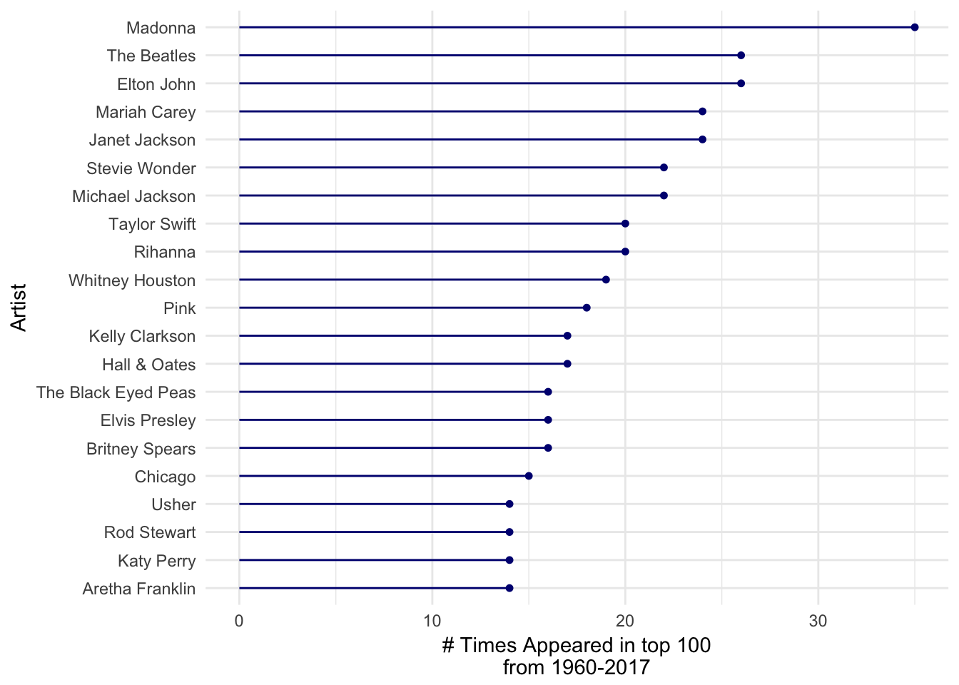
Now, I’m not exactly a musicologist, but I do enjoy my music. I gotta say, I wasn’t expecting:
- Madonna to beat the Beatles
- Elton John and The Beatles to be the same
- Janet Jackson to beat Michael Jackson
- Janet Jackson to be on par with Mariah Carey
- Britney Spears to be the same as Elvis
- The Black Eyed Peas to be the same as Elvis
And I gotta wonder, how did they get there? Was it a quick journey, a short one?
An artist’s rise to fame
Let’s see if we can view their rise to fame. We can keep a count of the number of times that an artist appeared in the top 100.
We then want to get a tally of the number of times that each artist appears. We can do this by grouping by the artist, arranging by artist and then year, and then creating a new variable that counts up from 1 to the number of times that artist appears. We also just chuck in a filter there to see what happens for just Madonna.
billboard_clean %>%
  # add a grouping category for the growth
  arrange(artist,year) %>%
  group_by(artist) %>%
  mutate(rank_tally = 1:n()) %>%
  ungroup() %>%
  filter(artist == "Madonna")
## # A tibble: 35 x 5
##     rank title             artist   year rank_tally
##    <dbl> <chr>             <chr>   <dbl>      <int>
##  1 35.0  Borderline        Madonna  1984          1
##  2 66.0  Lucky Star        Madonna  1984          2
##  3 79.0  Holiday           Madonna  1984          3
##  4  2.00 Like a Virgin     Madonna  1985          4
##  5  9.00 Crazy for You     Madonna  1985          5
##  6 58.0  Material Girl     Madonna  1985          6
##  7 81.0  Angel             Madonna  1985          7
##  8 98.0  Dress You Up      Madonna  1985          8
##  9 29.0  Papa Don't Preach Madonna  1986          9
## 10 35.0  Live to Tell      Madonna  1986         10
## # ... with 25 more rows
OK let’s put this in a new dataset, “billboard_clean_growth”
billboard_clean_growth <- billboard_clean %>%
  add_count(artist) %>%
  # add a grouping category for the growth
  arrange(artist,year) %>%
  group_by(artist) %>%
  mutate(rank_tally = 1:n()) %>%
  ungroup()
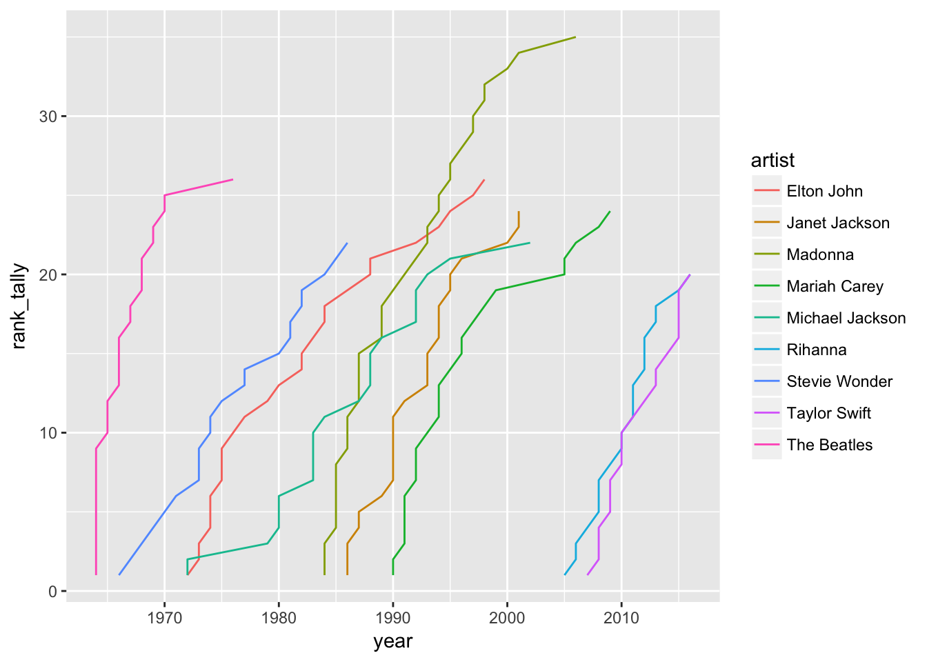
And now let’s visualise it, but let’s only look at those artists who appeared in the top 100 more than 20 times.
 billboard_clean_growth %>%
  filter(n >= 20) %>%
  ggplot(aes(x = year,
               y = rank_tally,
               group = artist,
               colour = artist)) +
    geom_line()
But let’s add some labels, and remove the legend.
 billboard_clean_growth %>%
  filter(n >= 21) %>%
  ggplot(aes(x = year,
               y = rank_tally,
               group = artist,
               colour = artist)) +
    geom_line() +
    geom_label(data = filter(billboard_clean_growth,
                             n >= 21,
                             rank_tally == n),
               aes(label = artist,
                   fill = artist),
               colour = "white") +
  theme_dark() +
  expand_limits(x = c(1964,2011)) +
  theme(legend.position = "none")
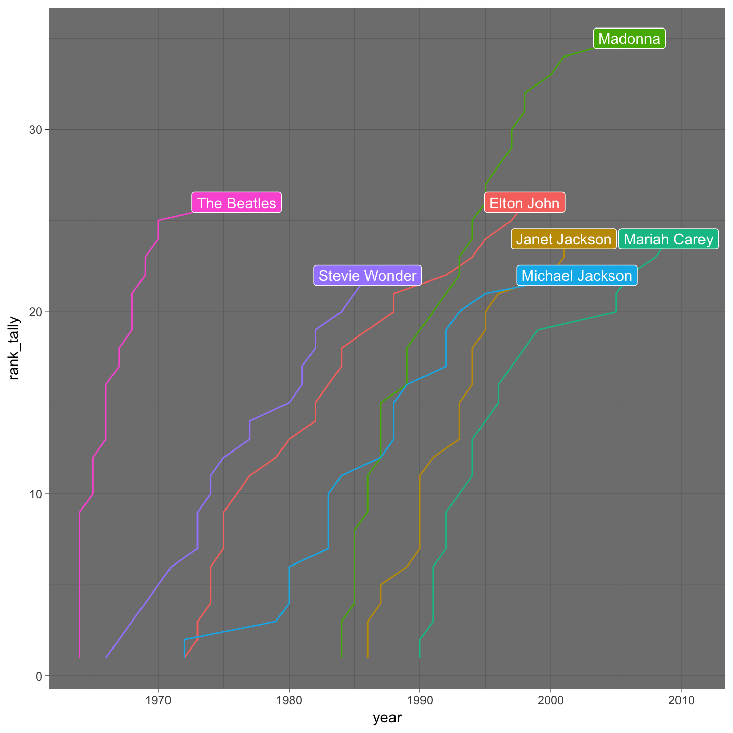
There you have it! The rise of artists over time.
Looking at this plot, it makes me want to investigate further with some kind of grouped/multi level growth model - identify those say with the most rapid growth, or perhaps the greatest predicted growth.
I guess the next logical step here is to look more at other kinds of music data - perhaps we can get information on the nationality of artists, and also combine together multiple databases - rolling stone, … and other labels.
There are also some other really cool datasets within the billboard package:
lyrics
A data set containing lyrics for songs on the Billboard Hot 100 over the past 57 years. The lyrics were identified and collected by webscraping so there might be some errors and mistakes - have that in mind.
spotify_track_data
A data set contaning 56 playlists from Spotify that were used to get the songs for the feature extraction of Billboard Hot 100 songs from 1960 to 2015 that you find in spotify_track_data.
spotify_playlists
Using the playlists in the spotify_playlists data set, this data contains the features of all of the tracks on the playlists.
Thanks again for making this R package, Mikkel Krogsholm - great stuff!
Conclusion
There you have it! Some (hopefully!) interesting data munging using tidyverse tools. I got to connect with some interesting music, and also learnt some cool stuff. Cool, right?
Spotify playlists: