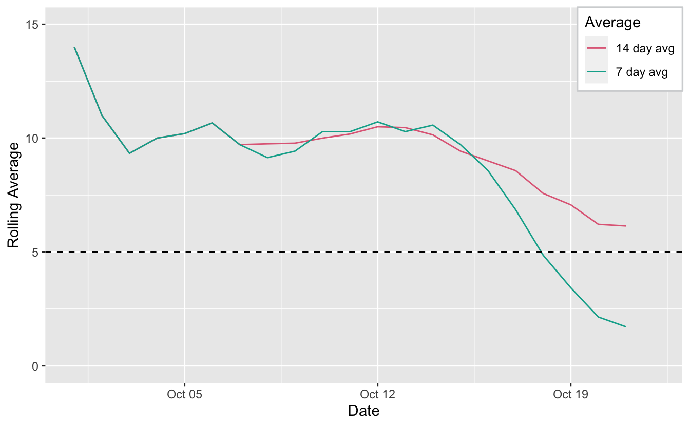
Things are moving along in the COVID19 world in Melbourne, and the latest numbers we are discussing are the 14 day and 7 day averages. The aim is to get the 14 day average below 5 cases, but people are starting to report the current 7 day average, since this is also encouraging and interesting.
So let’s explore how to do sliding averages. We’ll use the covid scraping code from a previous blog post on scraping covid data (I don’t think I’ll put this into yet another R package, but I’m tempted. But…anyway).
This code checks if we can scrape the data (bow()), scrapes the data (scrape()), extracts the tables (html_table()), picks (pluck) the second one, then converts it to a tibble for nice printing.
covidlive_url <- "https://covidlive.com.au/report/daily-cases/vic"

covidlive_raw <- covidlive_url %>%
  bow() %>%
  scrape() %>%
  html_table() %>%
  pluck(2) %>%
  as_tibble()
Then we do a bit of data cleaning, parsing the dates and numbers properly, and just leaving us with a date and case column:
strp_date <- function(x) as.Date(strptime(x, format = "%d %b"))

daily_cases <- covidlive_raw %>%
  mutate(DATE = strp_date(DATE),
         CASES = parse_number(CASES),
         NET = suppressWarnings(parse_number(NET))) %>%
  clean_names() %>%
  select(-var,
         -cases) %>%
  rename(cases = net) %>%
  select(date, cases)

daily_cases

#> # A tibble: 272 x 2
#>    date       cases
#>    <date>     <dbl>
#>  1 2020-10-22    NA
#>  2 2020-10-21     3
#>  3 2020-10-20     1
#>  4 2020-10-19     4
#>  5 2020-10-18    -2
#>  6 2020-10-17     0
#>  7 2020-10-16     2
#>  8 2020-10-15     4
#>  9 2020-10-14     6
#> 10 2020-10-13    10
#> # … with 262 more rows
We can then convert this into a tsibble, to make it easier to work with dates.
daily_ts <- as_tsibble(daily_cases,
                       index = date)
Sliding windows?
No we want to plot a 7 and 14 day average of cases. Thinking about how I would do this, I probably would have identified the “week” of a year, and then grouped by that and calculated the average, and maybe through some reduce/aggregate functional programming magic.
But there is now a more straightforward way, using using the {slider} R package by Davis Vaughn. This package allows for performing calculations on a specified window size. The idea is very powerful, and was in part inspired by the slide family of functions in tsibble.
Earo Wang has given some really nice explanations of what sliding is, in particular I like her JSM19 talk and rstudioconf::2019 talk - a visual representation is in this gif (lifted from Earo’s talk):
slider provides a more general interface, and draws upon the framework in purrr and vctrs R packages.
Let’s show an example by taking the last 14 days of covid cases
vec_cases <- daily_ts %>%
  tail(15) %>%
  pull(cases) %>%
  na.omit() %>%
  as.numeric()

vec_cases

#>  [1] 10 10 12 12 14 10  6  4  2  0 -2  4  1  3
We can use slide to calculate the mean of the last 7 days. We can demonstrate how this work by first just printing the data, and using the .before = 6, to print the previous 6 values, plus the current one:
slide(.x = vec_cases,
      .f = ~.x,
      .before = 6)

#> [[1]]
#> [1] 10
#>
#> [[2]]
#> [1] 10 10
#>
#> [[3]]
#> [1] 10 10 12
#>
#> [[4]]
#> [1] 10 10 12 12
#>
#> [[5]]
#> [1] 10 10 12 12 14
#>
#> [[6]]
#> [1] 10 10 12 12 14 10
#>
#> [[7]]
#> [1] 10 10 12 12 14 10  6
#>
#> [[8]]
#> [1] 10 12 12 14 10  6  4
#>
#> [[9]]
#> [1] 12 12 14 10  6  4  2
#>
#> [[10]]
#> [1] 12 14 10  6  4  2  0
#>
#> [[11]]
#> [1] 14 10  6  4  2  0 -2
#>
#> [[12]]
#> [1] 10  6  4  2  0 -2  4
#>
#> [[13]]
#> [1]  6  4  2  0 -2  4  1
#>
#> [[14]]
#> [1]  4  2  0 -2  4  1  3
This shows us 14 lists, the first 6 containing 1-6 of the numbers, then 7 from thereout.
We can instead run a function, like mean to calculate the mean on this output.
slide(.x = vec_cases,
      .f = mean,
      .before = 7)

#> [[1]]
#> [1] 10
#>
#> [[2]]
#> [1] 10
#>
#> [[3]]
#> [1] 10.66667
#>
#> [[4]]
#> [1] 11
#>
#> [[5]]
#> [1] 11.6
#>
#> [[6]]
#> [1] 11.33333
#>
#> [[7]]
#> [1] 10.57143
#>
#> [[8]]
#> [1] 9.75
#>
#> [[9]]
#> [1] 8.75
#>
#> [[10]]
#> [1] 7.5
#>
#> [[11]]
#> [1] 5.75
#>
#> [[12]]
#> [1] 4.75
#>
#> [[13]]
#> [1] 3.125
#>
#> [[14]]
#> [1] 2.25
We can even use the slide_dbl function to return these as all numeric (the type stability feature borrowed from purrr):
slide_dbl(.x = vec_cases,
          .f = mean,
          .before = 7)

#>  [1] 10.00000 10.00000 10.66667 11.00000 11.60000 11.33333 10.57143  9.75000
#>  [9]  8.75000  7.50000  5.75000  4.75000  3.12500  2.25000
Now let’s use this inside our data, first we filter the data down to from the start of october with filter_index("2020-10-01" ~ .), then, we calculate the average, using slide_index_dbl, where we specify the time index used in the data with i:
covid_rolls <- daily_ts %>%
  filter_index("2020-10-01" ~ .) %>%
  mutate(`7 day avg` = slide_index_dbl(.i = date,
                                .x = cases,
                                .f = mean,
                                .before = 6),
         `14 day avg` = slide_index_dbl(.i = date,
                                   .x = cases,
                                   .f = mean,
                                   .before = 13))

covid_rolls

#> # A tsibble: 22 x 4 [1D]
#>    date       cases `7 day avg` `14 day avg`
#>    <date>     <dbl>       <dbl>        <dbl>
#>  1 2020-10-01    14       14           14
#>  2 2020-10-02     8       11           11
#>  3 2020-10-03     6        9.33         9.33
#>  4 2020-10-04    12       10           10
#>  5 2020-10-05    11       10.2         10.2
#>  6 2020-10-06    13       10.7         10.7
#>  7 2020-10-07     4        9.71         9.71
#>  8 2020-10-08    10        9.14         9.75
#>  9 2020-10-09    10        9.43         9.78
#> 10 2020-10-10    12       10.3         10
#> # … with 12 more rows
We convert this into long form for easier plotting
covid_rolls_long <- covid_rolls %>%
  pivot_longer(cols = 3:4,
               names_to = "roll_type",
               values_to = "value")
covid_rolls_long

#> # A tsibble: 44 x 4 [1D]
#> # Key:       roll_type [2]
#>    date       cases roll_type  value
#>    <date>     <dbl> <chr>      <dbl>
#>  1 2020-10-01    14 7 day avg  14
#>  2 2020-10-01    14 14 day avg 14
#>  3 2020-10-02     8 7 day avg  11
#>  4 2020-10-02     8 14 day avg 11
#>  5 2020-10-03     6 7 day avg   9.33
#>  6 2020-10-03     6 14 day avg  9.33
#>  7 2020-10-04    12 7 day avg  10
#>  8 2020-10-04    12 14 day avg 10
#>  9 2020-10-05    11 7 day avg  10.2
#> 10 2020-10-05    11 14 day avg 10.2
#> # … with 34 more rows
Now let’s plot it!
ggplot(covid_rolls_long,
       aes(x = date,
           y = value,
           colour = roll_type)) +
  geom_line() +
  geom_hline(yintercept = 5, linetype = 2) +
  lims(y = c(0, 15)) +
  scale_colour_discrete_qualitative() +
  labs(x = "Date",
       y = "Rolling Average",
       colour = "Average") +
  # make the legend inset using code lifted from
  # https://github.com/MilesMcBain/inlegend/blob/master/R/legends.R
  theme(legend.justification = c(1, 1),
        legend.position = c(1.0, 1),
        legend.background = ggplot2::element_rect(
          colour = "#d3d5d6",
          fill = "#ffffff",
          size = 0.6
        ))

#> Warning: Removed 2 row(s) containing missing values (geom_path).
End
The slider R package is really neat, and there is more to say about it! But I just thought I’d finish by saying that it is indeed possible to do the same “stretch” and “tile” manouevers as provided by tsibble, and I would highly recommend checking out the slider website for more details on examples like rolling linear models and how to use it to perform row wise iteration.